核岭回归与高斯过程回归的比较#
本示例说明了核岭回归与高斯过程回归之间的差异。
核岭回归和高斯过程回归都使用所谓的“核技巧”来使它们的模型具有足够的表达能力以拟合训练数据。但是,这两种方法解决的机器学习问题截然不同。
核岭回归将找到最小化损失函数(均方误差)的目标函数。
高斯过程回归不是找到单个目标函数,而是采用概率方法:基于贝叶斯定理定义目标函数上的高斯后验分布,因此目标函数的先验概率与观察到的训练数据定义的似然函数相结合,以提供后验分布的估计。
我们将通过一个例子来说明这些差异,我们还将重点关注调整核超参数。
# Authors: Jan Hendrik Metzen <jhm@informatik.uni-bremen.de>
#          Guillaume Lemaitre <g.lemaitre58@gmail.com>
# License: BSD 3 clause
生成数据集#
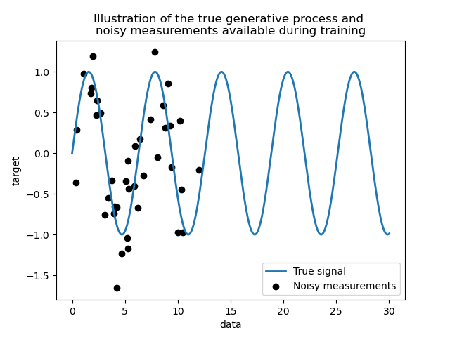
我们创建一个合成数据集。真实的生成过程将采用一个一维向量并计算其正弦值。请注意,此正弦的周期因此为 \(2 \pi\)。我们将在本示例的后面部分重用此信息。
import numpy as np

rng = np.random.RandomState(0)
data = np.linspace(0, 30, num=1_000).reshape(-1, 1)
target = np.sin(data).ravel()
现在,我们可以想象一个我们从这个真实过程中获得观察结果的场景。但是,我们将添加一些挑战
测量结果将包含噪声;
只有信号开始部分的样本可用。
training_sample_indices = rng.choice(np.arange(0, 400), size=40, replace=False)
training_data = data[training_sample_indices]
training_noisy_target = target[training_sample_indices] + 0.5 * rng.randn(
    len(training_sample_indices)
)
让我们绘制真实信号和可用于训练的噪声测量值。
import matplotlib.pyplot as plt

plt.plot(data, target, label="True signal", linewidth=2)
plt.scatter(
    training_data,
    training_noisy_target,
    color="black",
    label="Noisy measurements",
)
plt.legend()
plt.xlabel("data")
plt.ylabel("target")
_ = plt.title(
    "Illustration of the true generative process and \n"
    "noisy measurements available during training"
)
简单线性模型的局限性#
首先,我们想强调一下线性模型在给定数据集上的局限性。我们拟合了一个 Ridge 并检查该模型在我们的数据集上的预测。
from sklearn.linear_model import Ridge

ridge = Ridge().fit(training_data, training_noisy_target)

plt.plot(data, target, label="True signal", linewidth=2)
plt.scatter(
    training_data,
    training_noisy_target,
    color="black",
    label="Noisy measurements",
)
plt.plot(data, ridge.predict(data), label="Ridge regression")
plt.legend()
plt.xlabel("data")
plt.ylabel("target")
_ = plt.title("Limitation of a linear model such as ridge")
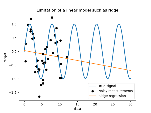
这种岭回归器欠拟合数据,因为它没有足够的表达能力。
核方法:核岭和高斯过程#
核岭#
我们可以通过使用所谓的核来使先前的线性模型更具表达力。核是从原始特征空间到另一个特征空间的嵌入。简而言之,它用于将我们的原始数据映射到一个更新、更复杂的特征空间中。这个新空间由核的选择明确定义。
在我们的例子中,我们知道真实的生成过程是一个周期函数。我们可以使用一个 ExpSineSquared 核,它允许恢复周期性。 KernelRidge 类将接受这样的核。
将此模型与核一起使用等效于使用核的映射函数嵌入数据,然后应用岭回归。在实践中,数据不会被显式映射;相反,使用“核技巧”计算更高维特征空间中样本之间的点积。
因此,让我们使用这样的 KernelRidge。
import time

from sklearn.gaussian_process.kernels import ExpSineSquared
from sklearn.kernel_ridge import KernelRidge

kernel_ridge = KernelRidge(kernel=ExpSineSquared())

start_time = time.time()
kernel_ridge.fit(training_data, training_noisy_target)
print(
    f"Fitting KernelRidge with default kernel: {time.time() - start_time:.3f} seconds"
)
Fitting KernelRidge with default kernel: 0.001 seconds
plt.plot(data, target, label="True signal", linewidth=2, linestyle="dashed")
plt.scatter(
    training_data,
    training_noisy_target,
    color="black",
    label="Noisy measurements",
)
plt.plot(
    data,
    kernel_ridge.predict(data),
    label="Kernel ridge",
    linewidth=2,
    linestyle="dashdot",
)
plt.legend(loc="lower right")
plt.xlabel("data")
plt.ylabel("target")
_ = plt.title(
    "Kernel ridge regression with an exponential sine squared\n "
    "kernel using default hyperparameters"
)
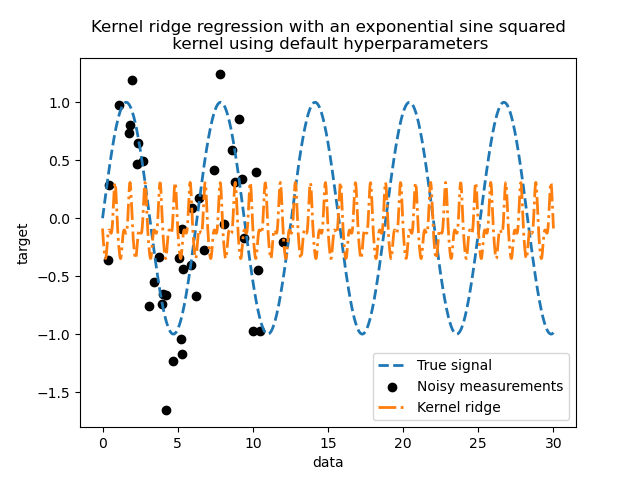
这个拟合模型不准确。事实上,我们没有设置核的参数,而是使用了默认的参数。我们可以检查它们。
kernel_ridge.kernel
ExpSineSquared(length_scale=1, periodicity=1)
我们的核有两个参数:长度尺度和周期性。对于我们的数据集,我们使用 sin 作为生成过程,这意味着信号的周期为 \(2 \pi\)。参数的默认值为 \(1\),这解释了在我们的模型预测中观察到的高频。可以使用长度尺度参数得出类似的结论。因此,它告诉我们核参数需要调整。我们将使用随机搜索来调整核岭模型的不同参数:alpha 参数和核参数。
from scipy.stats import loguniform

from sklearn.model_selection import RandomizedSearchCV

param_distributions = {
    "alpha": loguniform(1e0, 1e3),
    "kernel__length_scale": loguniform(1e-2, 1e2),
    "kernel__periodicity": loguniform(1e0, 1e1),
}
kernel_ridge_tuned = RandomizedSearchCV(
    kernel_ridge,
    param_distributions=param_distributions,
    n_iter=500,
    random_state=0,
)
start_time = time.time()
kernel_ridge_tuned.fit(training_data, training_noisy_target)
print(f"Time for KernelRidge fitting: {time.time() - start_time:.3f} seconds")
Time for KernelRidge fitting: 4.643 seconds
现在拟合模型的计算成本更高,因为我们必须尝试超参数的几种组合。我们可以看看找到的超参数以获得一些直觉。
kernel_ridge_tuned.best_params_
{'alpha': 1.9915849773450223, 'kernel__length_scale': 0.7986499491396727, 'kernel__periodicity': 6.607275806426107}
查看最佳参数,我们发现它们与默认值不同。我们还看到周期性更接近预期值:\(2 \pi\)。我们现在可以检查我们调整后的核岭的预测。
Time for KernelRidge predict: 0.002 seconds
plt.plot(data, target, label="True signal", linewidth=2, linestyle="dashed")
plt.scatter(
    training_data,
    training_noisy_target,
    color="black",
    label="Noisy measurements",
)
plt.plot(
    data,
    predictions_kr,
    label="Kernel ridge",
    linewidth=2,
    linestyle="dashdot",
)
plt.legend(loc="lower right")
plt.xlabel("data")
plt.ylabel("target")
_ = plt.title(
    "Kernel ridge regression with an exponential sine squared\n "
    "kernel using tuned hyperparameters"
)
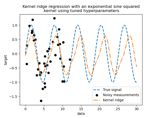
我们得到了一个更准确的模型。我们仍然观察到一些错误,主要是由于添加到数据集中的噪声。
高斯过程回归#
现在,我们将使用 GaussianProcessRegressor 来拟合相同的数据集。在训练高斯过程时,核的超参数在拟合过程中被优化。不需要外部超参数搜索。在这里,我们创建了一个比核岭回归器稍微复杂的核:我们添加了一个 WhiteKernel,用于估计数据集中的噪声。
from sklearn.gaussian_process import GaussianProcessRegressor
from sklearn.gaussian_process.kernels import WhiteKernel

kernel = 1.0 * ExpSineSquared(1.0, 5.0, periodicity_bounds=(1e-2, 1e1)) + WhiteKernel(
    1e-1
)
gaussian_process = GaussianProcessRegressor(kernel=kernel)
start_time = time.time()
gaussian_process.fit(training_data, training_noisy_target)
print(
    f"Time for GaussianProcessRegressor fitting: {time.time() - start_time:.3f} seconds"
)
Time for GaussianProcessRegressor fitting: 0.031 seconds
训练高斯过程的计算成本远低于使用随机搜索的核岭。我们可以检查我们计算的核的参数。
gaussian_process.kernel_
0.675**2 * ExpSineSquared(length_scale=1.34, periodicity=6.57) + WhiteKernel(noise_level=0.182)
事实上,我们看到参数已经过优化。查看 periodicity 参数,我们发现我们找到了一个接近理论值 \(2 \pi\) 的周期。我们现在可以看看我们模型的预测。
Time for GaussianProcessRegressor predict: 0.002 seconds
plt.plot(data, target, label="True signal", linewidth=2, linestyle="dashed")
plt.scatter(
    training_data,
    training_noisy_target,
    color="black",
    label="Noisy measurements",
)
# Plot the predictions of the kernel ridge
plt.plot(
    data,
    predictions_kr,
    label="Kernel ridge",
    linewidth=2,
    linestyle="dashdot",
)
# Plot the predictions of the gaussian process regressor
plt.plot(
    data,
    mean_predictions_gpr,
    label="Gaussian process regressor",
    linewidth=2,
    linestyle="dotted",
)
plt.fill_between(
    data.ravel(),
    mean_predictions_gpr - std_predictions_gpr,
    mean_predictions_gpr + std_predictions_gpr,
    color="tab:green",
    alpha=0.2,
)
plt.legend(loc="lower right")
plt.xlabel("data")
plt.ylabel("target")
_ = plt.title("Comparison between kernel ridge and gaussian process regressor")
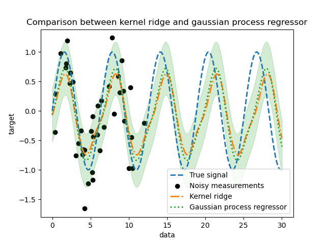
我们观察到核岭和高斯过程回归器的结果很接近。但是,高斯过程回归器还提供了核岭无法提供的 uncertainty 信息。由于目标函数的概率公式,高斯过程可以输出标准偏差(或协方差)以及目标函数的均值预测。
但是,这是有代价的:使用高斯过程计算预测的时间更长。
最终结论#
我们可以就两种模型外推的可能性给出最后一句话。事实上,我们只提供了信号的开头作为训练集。使用周期性核强制我们的模型重复在训练集中找到的模式。使用此核信息以及两种模型外推的能力,我们观察到模型将继续预测正弦模式。
高斯过程允许将核组合在一起。因此,我们可以将指数正弦平方核与径向基函数核关联起来。
from sklearn.gaussian_process.kernels import RBF

kernel = 1.0 * ExpSineSquared(1.0, 5.0, periodicity_bounds=(1e-2, 1e1)) * RBF(
    length_scale=15, length_scale_bounds="fixed"
) + WhiteKernel(1e-1)
gaussian_process = GaussianProcessRegressor(kernel=kernel)
gaussian_process.fit(training_data, training_noisy_target)
mean_predictions_gpr, std_predictions_gpr = gaussian_process.predict(
    data,
    return_std=True,
)
plt.plot(data, target, label="True signal", linewidth=2, linestyle="dashed")
plt.scatter(
    training_data,
    training_noisy_target,
    color="black",
    label="Noisy measurements",
)
# Plot the predictions of the kernel ridge
plt.plot(
    data,
    predictions_kr,
    label="Kernel ridge",
    linewidth=2,
    linestyle="dashdot",
)
# Plot the predictions of the gaussian process regressor
plt.plot(
    data,
    mean_predictions_gpr,
    label="Gaussian process regressor",
    linewidth=2,
    linestyle="dotted",
)
plt.fill_between(
    data.ravel(),
    mean_predictions_gpr - std_predictions_gpr,
    mean_predictions_gpr + std_predictions_gpr,
    color="tab:green",
    alpha=0.2,
)
plt.legend(loc="lower right")
plt.xlabel("data")
plt.ylabel("target")
_ = plt.title("Effect of using a radial basis function kernel")
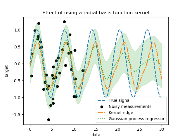
一旦训练中没有样本可用,使用径向基函数核的效果将减弱周期性效应。随着测试样本越来越远离训练样本,预测会收敛到它们的均值,并且它们的标准偏差也会增加。
脚本总运行时间:(0 分 5.413 秒)
相关示例