7.6. 随机投影#
sklearn.random_projection 模块实现了一种简单且计算高效的方法来降低数据维度,它以牺牲一定可控的精度(作为额外的方差)来换取更快的处理速度和更小的模型大小。该模块实现了两种非结构化的随机矩阵:高斯随机矩阵 和 稀疏随机矩阵。
随机投影矩阵的维度和分布经过控制,以保留数据集中任意两个样本之间的成对距离。因此,随机投影是一种适用于基于距离的方法的近似技术。
References
Sanjoy Dasgupta. 2000. Experiments with random projection. In Proceedings of the Sixteenth conference on Uncertainty in artificial intelligence (UAI’00), Craig Boutilier and Moisés Goldszmidt (Eds.). Morgan Kaufmann Publishers Inc., San Francisco, CA, USA, 143-151.
Ella Bingham and Heikki Mannila. 2001. Random projection in dimensionality reduction: applications to image and text data. In Proceedings of the seventh ACM SIGKDD international conference on Knowledge discovery and data mining (KDD ‘01). ACM, New York, NY, USA, 245-250.
7.6.1. Johnson-Lindenstrauss 引理#
随机投影效率背后的主要理论结果是 Johnson-Lindenstrauss 引理 (引用自维基百科)
在数学中,Johnson-Lindenstrauss 引理是关于将点从高维欧几里得空间低失真嵌入到低维欧几里得空间的结果。该引理指出,高维空间中的一小组点可以嵌入到维度低得多的空间中,且点之间的距离几乎得以保留。用于嵌入的映射至少是 Lipschitz 连续的,并且可以被视为正交投影。
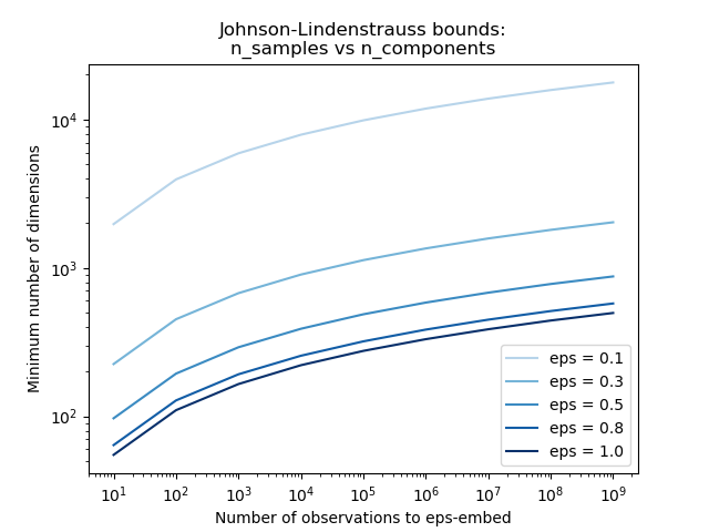
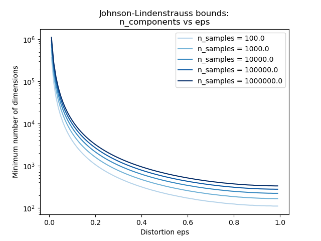
仅知道样本数量,johnson_lindenstrauss_min_dim 会保守地估计随机子空间的最小大小,以保证随机投影引入的有界失真
>>> from sklearn.random_projection import johnson_lindenstrauss_min_dim
>>> johnson_lindenstrauss_min_dim(n_samples=1e6, eps=0.5)
np.int64(663)
>>> johnson_lindenstrauss_min_dim(n_samples=1e6, eps=[0.5, 0.1, 0.01])
array([    663,   11841, 1112658])
>>> johnson_lindenstrauss_min_dim(n_samples=[1e4, 1e5, 1e6], eps=0.1)
array([ 7894,  9868, 11841])
示例
请参阅 Johnson-Lindenstrauss bound for embedding with random projections,了解关于 Johnson-Lindenstrauss 引理的理论解释以及使用稀疏随机矩阵进行的经验验证。
References
Sanjoy Dasgupta and Anupam Gupta, 1999. An elementary proof of the Johnson-Lindenstrauss Lemma.
7.6.2. 高斯随机投影#
GaussianRandomProjection 通过将原始输入空间投影到一个随机生成的矩阵上以降低维度,该矩阵的分量是从分布 \(N(0, \frac{1}{n_{components}})\) 中抽取的。
下面是一个小片段,演示了如何使用高斯随机投影变换器
>>> import numpy as np
>>> from sklearn import random_projection
>>> X = np.random.rand(100, 10000)
>>> transformer = random_projection.GaussianRandomProjection()
>>> X_new = transformer.fit_transform(X)
>>> X_new.shape
(100, 3947)
7.6.3. 稀疏随机投影#
SparseRandomProjection 通过使用稀疏随机矩阵投影原始输入空间来降低维度。
稀疏随机矩阵是密集高斯随机投影矩阵的替代方案,它保证了相似的嵌入质量,同时内存效率更高,并且允许更快地计算投影数据。
如果我们定义 s = 1 / density,随机矩阵的元素从以下分布中抽取
其中 \(n_{\text{components}}\) 是投影子空间的大小。默认情况下,非零元素的密度设置为 Ping Li 等人推荐的最小密度:\(1 / \sqrt{n_{\text{features}}}\)。
下面是一个小片段,演示了如何使用稀疏随机投影变换器
>>> import numpy as np
>>> from sklearn import random_projection
>>> X = np.random.rand(100, 10000)
>>> transformer = random_projection.SparseRandomProjection()
>>> X_new = transformer.fit_transform(X)
>>> X_new.shape
(100, 3947)
References
D. Achlioptas. 2003. Database-friendly random projections: Johnson-Lindenstrauss with binary coins. Journal of Computer and System Sciences 66 (2003) 671-687.
Ping Li, Trevor J. Hastie, and Kenneth W. Church. 2006. Very sparse random projections. In Proceedings of the 12th ACM SIGKDD international conference on Knowledge discovery and data mining (KDD ‘06). ACM, New York, NY, USA, 287-296.
7.6.4. 逆变换#
随机投影变换器具有 compute_inverse_components 参数。当设置为 True 时,在拟合期间创建随机 components_ 矩阵后,变换器会计算此矩阵的伪逆,并将其存储为 inverse_components_。inverse_components_ 矩阵的形状为 \(n_{features} \times n_{components}\),并且它始终是一个密集矩阵,无论 components 矩阵是稀疏还是密集。因此,根据特征数和分量数,它可能会占用大量内存。
当调用 inverse_transform 方法时,它会计算输入 X 与逆分量转置的乘积。如果在拟合期间已经计算了逆分量,则在每次调用 inverse_transform 时都会重用它们。否则,每次都会重新计算,这可能会很耗时。即使 X 是稀疏的,结果也始终是密集的。
下面是一个小代码示例,演示了如何使用逆变换功能
>>> import numpy as np
>>> from sklearn.random_projection import SparseRandomProjection
>>> X = np.random.rand(100, 10000)
>>> transformer = SparseRandomProjection(
...   compute_inverse_components=True
... )
...
>>> X_new = transformer.fit_transform(X)
>>> X_new.shape
(100, 3947)
>>> X_new_inversed = transformer.inverse_transform(X_new)
>>> X_new_inversed.shape
(100, 10000)
>>> X_new_again = transformer.transform(X_new_inversed)
>>> np.allclose(X_new, X_new_again)
True