6. 可视化#
Scikit-learn 定义了一个简单的 API,用于创建机器学习的可视化。此 API 的关键特性是允许快速绘图和视觉调整,而无需重新计算。我们提供了 Display 类,这些类公开了两种创建图表的方法:from_estimator 和 from_predictions。
from_estimator 方法从一个已拟合的估计器、输入数据(X、y)和一个图表生成一个 Display 对象。from_predictions 方法从真实值和预测值(y_test、y_pred)和一个图表创建 Display 对象。
使用 from_predictions 可以避免重新计算预测,但用户需要注意传递的预测值与 pos_label 相对应。对于 predict_proba,选择与 pos_label 类对应的列;而对于 decision_function,如果 pos_label 不是估计器 classes_ 属性中的最后一个类,则反转分数(即乘以 -1)。
Display 对象存储了使用 Matplotlib 绘图所需的计算值(例如,指标值或特征重要性)。这些值是从传递给 from_predictions 的原始预测,或传递给 from_estimator 的估计器和 X 中得出的结果。
一旦 Display 对象被初始化(请注意,我们建议通过 from_estimator 或 from_predictions 而不是直接初始化来创建 Display 对象),它就具有一个 plot 方法来创建 Matplotlib 图表。plot 方法允许通过将现有图表的 matplotlib.axes.Axes 传递给 ax 参数来添加到现有图表。
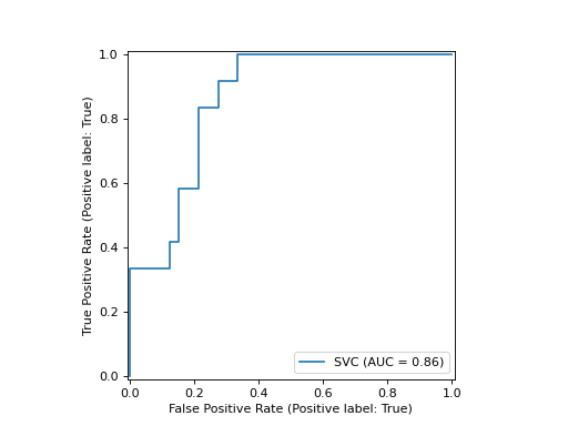
在下面的示例中,我们使用 from_estimator 为已拟合的 Logistic Regression 模型绘制 ROC 曲线
from sklearn.model_selection import train_test_split
from sklearn.linear_model import LogisticRegression
from sklearn.metrics import RocCurveDisplay
from sklearn.datasets import load_iris

X, y = load_iris(return_X_y=True)
y = y == 2  # make binary
X_train, X_test, y_train, y_test = train_test_split(
   X, y, test_size=.8, random_state=42
)
clf = LogisticRegression(random_state=42, C=.01)
clf.fit(X_train, y_train)

clf_disp = RocCurveDisplay.from_estimator(clf, X_test, y_test)
如果您已经有了预测值,您可以改用 from_predictions 来做同样的事情(并节省计算量)
from sklearn.model_selection import train_test_split
from sklearn.linear_model import LogisticRegression
from sklearn.metrics import RocCurveDisplay
from sklearn.datasets import load_iris

X, y = load_iris(return_X_y=True)
y = y == 2  # make binary
X_train, X_test, y_train, y_test = train_test_split(
   X, y, test_size=.8, random_state=42
)
clf = LogisticRegression(random_state=42, C=.01)
clf.fit(X_train, y_train)

# select the probability of the class that we considered to be the positive label
y_pred = clf.predict_proba(X_test)[:, 1]

clf_disp = RocCurveDisplay.from_predictions(y_test, y_pred)
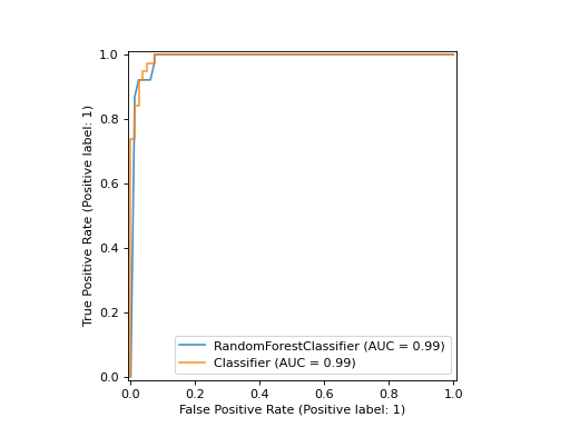
返回的 clf_disp 对象允许我们在已计算的 ROC 曲线中添加另一条曲线。在这种情况下,clf_disp 是一个 RocCurveDisplay,它将计算值存储为属性 roc_auc、fpr 和 tpr。
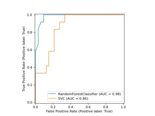
接下来,我们训练一个随机森林分类器,并通过使用 Display 对象的 plot 方法再次绘制之前计算的 ROC 曲线。
import matplotlib.pyplot as plt
from sklearn.ensemble import RandomForestClassifier

rfc = RandomForestClassifier(n_estimators=10, random_state=42)
rfc.fit(X_train, y_train)

ax = plt.gca()
rfc_disp = RocCurveDisplay.from_estimator(
  rfc, X_test, y_test, ax=ax, curve_kwargs={"alpha": 0.8}
)
clf_disp.plot(ax=ax, curve_kwargs={"alpha": 0.8})
请注意,我们将 alpha=0.8 传递给 plot 函数以调整曲线的 alpha 值。
示例
6.1. 可用的绘图工具#
6.1.1. Display 对象#
|
校准曲线(也称为可靠性图)可视化。 |
|
部分依赖图 (PDP) 和个体条件期望 (ICE)。 |
|
决策边界可视化。 |
|
混淆矩阵可视化。 |
|
检测错误权衡 (DET) 曲线可视化。 |
|
精确度-召回率可视化。 |
|
回归模型预测误差的可视化。 |
|
ROC 曲线可视化。 |
学习曲线可视化。 |
|
验证曲线可视化。 |