带结构和不带结构的层次聚类

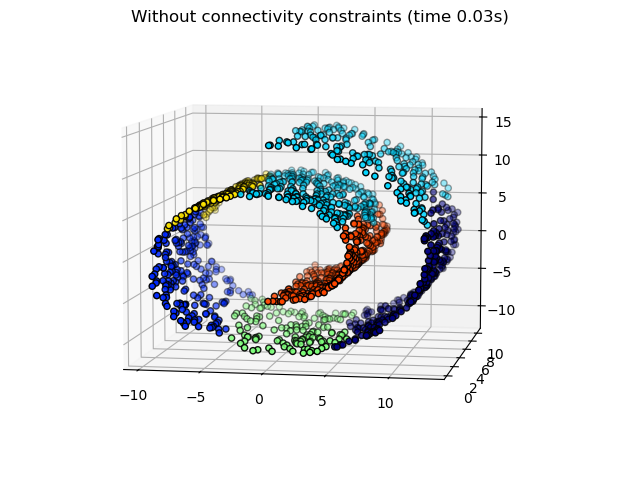
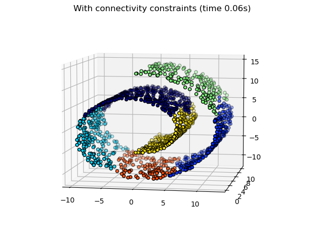
此示例演示了有无连通性约束的层次聚类。它展示了施加连通性图来捕获数据中局部结构的效果。没有连通性约束时，聚类纯粹基于距离；而有约束时，聚类会尊重局部结构。

更多信息请参见层次聚类。

施加连通性有两个优点。首先，使用稀疏连通性矩阵进行聚类通常更快。

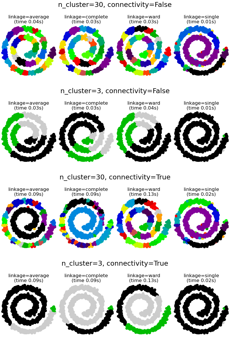
其次，当使用连通性矩阵时，single、average和complete linkage是不稳定的，并且倾向于创建一些增长非常快的簇。确实，average和complete linkage通过在合并簇时考虑两个簇之间的所有距离来对抗这种渗流行为（而single linkage通过仅考虑簇之间的最短距离来夸大这种行为）。连通性图打破了 average 和 complete linkage 的这种机制，使它们更类似于更脆弱的 single linkage。对于非常稀疏的图（尝试减少kneighbors_graph中的邻居数量）和 complete linkage，这种效果更为明显。特别是，图中邻居数量非常少时，施加的几何形状接近于 single linkage，而 single linkage 众所周知存在这种渗流不稳定性。

施加连通性的效果在两个不同但相似的数据集上进行了说明，它们都显示出螺旋结构。在第一个示例中，我们构建了一个 Swiss roll 数据集，并对其数据位置运行层次聚类。在这里，我们将非结构化的 Ward 聚类与强制执行 k-近邻连通性的结构化变体进行了比较。在第二个示例中，我们展示了将这种连通性图应用于 single、average 和 complete linkage 的效果。

# Authors: The scikit-learn developers
# SPDX-License-Identifier: BSD-3-Clause

生成 Swiss Roll 数据集。

import time

from sklearn.cluster import AgglomerativeClustering
from sklearn.datasets import make_swiss_roll

n_samples = 1500
noise = 0.05
X1, _ = make_swiss_roll(n_samples, noise=noise)
X1[:, 1] *= 0.5  # Make the roll thinner

计算无连通性约束的聚类

print("Compute unstructured hierarchical clustering...")
st = time.time()
ward_unstructured = AgglomerativeClustering(n_clusters=6, linkage="ward").fit(X1)
elapsed_time_unstructured = time.time() - st
label_unstructured = ward_unstructured.labels_
print(f"Elapsed time: {elapsed_time_unstructured:.2f}s")
print(f"Number of points: {label_unstructured.size}")

Compute unstructured hierarchical clustering...
Elapsed time: 0.03s
Number of points: 1500

绘制非结构化聚类结果

import matplotlib.pyplot as plt
import numpy as np

fig1 = plt.figure()
ax1 = fig1.add_subplot(111, projection="3d", elev=7, azim=-80)
ax1.set_position([0, 0, 0.95, 1])
for l in np.unique(label_unstructured):
    ax1.scatter(
        X1[label_unstructured == l, 0],
        X1[label_unstructured == l, 1],
        X1[label_unstructured == l, 2],
        color=plt.cm.jet(float(l) / np.max(label_unstructured + 1)),
        s=20,
        edgecolor="k",
    )
_ = fig1.suptitle(
    f"Without connectivity constraints (time {elapsed_time_unstructured:.2f}s)"
)

计算有连通性约束的聚类

from sklearn.neighbors import kneighbors_graph

connectivity = kneighbors_graph(X1, n_neighbors=10, include_self=False)

print("Compute structured hierarchical clustering...")
st = time.time()
ward_structured = AgglomerativeClustering(
    n_clusters=6, connectivity=connectivity, linkage="ward"
).fit(X1)
elapsed_time_structured = time.time() - st
label_structured = ward_structured.labels_
print(f"Elapsed time: {elapsed_time_structured:.2f}s")
print(f"Number of points: {label_structured.size}")

Compute structured hierarchical clustering...
Elapsed time: 0.06s
Number of points: 1500

绘制结构化聚类结果

fig2 = plt.figure()
ax2 = fig2.add_subplot(111, projection="3d", elev=7, azim=-80)
ax2.set_position([0, 0, 0.95, 1])
for l in np.unique(label_structured):
    ax2.scatter(
        X1[label_structured == l, 0],
        X1[label_structured == l, 1],
        X1[label_structured == l, 2],
        color=plt.cm.jet(float(l) / np.max(label_structured + 1)),
        s=20,
        edgecolor="k",
    )
_ = fig2.suptitle(
    f"With connectivity constraints (time {elapsed_time_structured:.2f}s)"
)

生成二维螺旋数据集。

n_samples = 1500
np.random.seed(0)
t = 1.5 * np.pi * (1 + 3 * np.random.rand(1, n_samples))
x = t * np.cos(t)
y = t * np.sin(t)

X2 = np.concatenate((x, y))
X2 += 0.7 * np.random.randn(2, n_samples)
X2 = X2.T

使用图捕获局部连通性

邻居数量越多，聚类越均匀，但计算时间成本越高。非常多的邻居数量会使聚类大小分布更均匀，但可能无法施加数据的局部流形结构。

knn_graph = kneighbors_graph(X2, 30, include_self=False)

绘制有结构和无结构的聚类

fig3 = plt.figure(figsize=(8, 12))
subfigs = fig3.subfigures(4, 1)
params = [
    (None, 30),
    (None, 3),
    (knn_graph, 30),
    (knn_graph, 3),
]

for subfig, (connectivity, n_clusters) in zip(subfigs, params):
    axs = subfig.subplots(1, 4, sharey=True)
    for index, linkage in enumerate(("average", "complete", "ward", "single")):
        model = AgglomerativeClustering(
            linkage=linkage, connectivity=connectivity, n_clusters=n_clusters
        )
        t0 = time.time()
        model.fit(X2)
        elapsed_time = time.time() - t0
        axs[index].scatter(
            X2[:, 0], X2[:, 1], c=model.labels_, cmap=plt.cm.nipy_spectral
        )
        axs[index].set_title(
            "linkage=%s\n(time %.2fs)" % (linkage, elapsed_time),
            fontdict=dict(verticalalignment="top"),
        )
        axs[index].set_aspect("equal")
        axs[index].axis("off")

        subfig.subplots_adjust(bottom=0, top=0.83, wspace=0, left=0, right=1)
        subfig.suptitle(
            "n_cluster=%i, connectivity=%r" % (n_clusters, connectivity is not None),
            size=17,
        )

plt.show()

相关示例

对硬币图像进行结构化 Ward 分层聚类演示

对硬币图像进行结构化 Ward 分层聚类演示

在玩具数据集上比较不同的分层链接方法

在玩具数据集上比较不同的分层链接方法

在数字的 2D 嵌入上进行各种 Agglomerative 聚类

在数字的 2D 嵌入上进行各种 Agglomerative 聚类

在玩具数据集上比较不同的聚类算法

在玩具数据集上比较不同的聚类算法