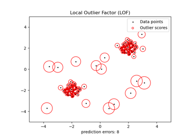
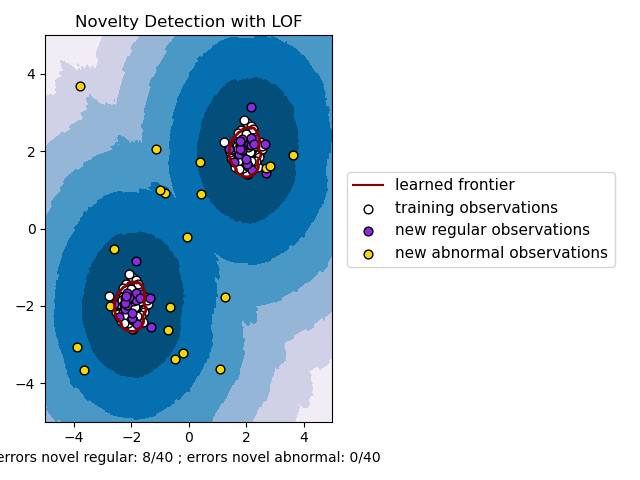
使用 Local Outlier Factor (LOF) 进行新颖性检测#

Local Outlier Factor (LOF) 算法是一种无监督的异常检测方法，它计算给定数据点相对于其邻居的局部密度偏差。它将密度远低于其邻居的样本视为异常值。此示例展示了如何使用 LOF 进行新颖性检测。请注意，当 LOF 用于新颖性检测时，您**绝不能**在训练集上使用 predict、decision_function 和 score_samples，因为这会导致错误的结果。您只能对新的未见数据（不在训练集中的数据）使用这些方法。有关异常值检测和新颖性检测之间区别以及如何使用 LOF 进行异常值检测的详细信息，请参阅用户指南。

考虑的邻居数量（参数 n_neighbors）通常设置为 1) 大于一个簇必须包含的最小样本数，以便其他样本可以相对于该簇成为局部异常值，以及 2) 小于可能成为局部异常值的附近样本的最大数量。在实践中，此类信息通常不可用，并且通常采用 n_neighbors=20 效果很好。

# Authors: The scikit-learn developers
# SPDX-License-Identifier: BSD-3-Clause

import matplotlib
import matplotlib.lines as mlines
import matplotlib.pyplot as plt
import numpy as np

from sklearn.neighbors import LocalOutlierFactor

np.random.seed(42)

xx, yy = np.meshgrid(np.linspace(-5, 5, 500), np.linspace(-5, 5, 500))
# Generate normal (not abnormal) training observations
X = 0.3 * np.random.randn(100, 2)
X_train = np.r_[X + 2, X - 2]
# Generate new normal (not abnormal) observations
X = 0.3 * np.random.randn(20, 2)
X_test = np.r_[X + 2, X - 2]
# Generate some abnormal novel observations
X_outliers = np.random.uniform(low=-4, high=4, size=(20, 2))

# fit the model for novelty detection (novelty=True)
clf = LocalOutlierFactor(n_neighbors=20, novelty=True, contamination=0.1)
clf.fit(X_train)
# DO NOT use predict, decision_function and score_samples on X_train as this
# would give wrong results but only on new unseen data (not used in X_train),
# e.g. X_test, X_outliers or the meshgrid
y_pred_test = clf.predict(X_test)
y_pred_outliers = clf.predict(X_outliers)
n_error_test = y_pred_test[y_pred_test == -1].size
n_error_outliers = y_pred_outliers[y_pred_outliers == 1].size

# plot the learned frontier, the points, and the nearest vectors to the plane
Z = clf.decision_function(np.c_[xx.ravel(), yy.ravel()])
Z = Z.reshape(xx.shape)

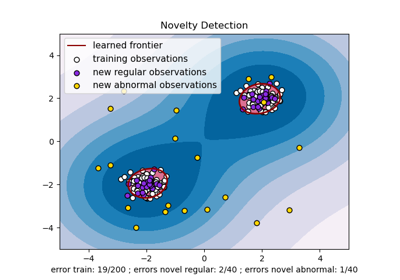
plt.title("Novelty Detection with LOF")
plt.contourf(xx, yy, Z, levels=np.linspace(Z.min(), 0, 7), cmap=plt.cm.PuBu)
a = plt.contour(xx, yy, Z, levels=[0], linewidths=2, colors="darkred")
plt.contourf(xx, yy, Z, levels=[0, Z.max()], colors="palevioletred")

s = 40
b1 = plt.scatter(X_train[:, 0], X_train[:, 1], c="white", s=s, edgecolors="k")
b2 = plt.scatter(X_test[:, 0], X_test[:, 1], c="blueviolet", s=s, edgecolors="k")
c = plt.scatter(X_outliers[:, 0], X_outliers[:, 1], c="gold", s=s, edgecolors="k")
plt.axis("tight")
plt.xlim((-5, 5))
plt.ylim((-5, 5))
plt.legend(
    [mlines.Line2D([], [], color="darkred"), b1, b2, c],
    [
        "learned frontier",
        "training observations",
        "new regular observations",
        "new abnormal observations",
    ],
    loc=(1.05, 0.4),
    prop=matplotlib.font_manager.FontProperties(size=11),
)
plt.xlabel(
    "errors novel regular: %d/40 ; errors novel abnormal: %d/40"
    % (n_error_test, n_error_outliers)
)
plt.tight_layout()
plt.show()

脚本总运行时间： (0 minutes 0.705 seconds)

使用 Local Outlier Factor (LOF) 进行新颖性检测#

本页