注意
跳到末尾 下载完整的示例代码,或通过 JupyterLite 或 Binder 在浏览器中运行此示例。
高斯混合模型选择#
本示例展示了如何使用高斯混合模型(GMM)通过信息论准则进行模型选择。模型选择涉及协方差类型和模型中的组件数量。
在这种情况下,赤池信息准则(AIC)和贝叶斯信息准则(BIC)都提供了正确的结果,但我们只演示后者,因为 BIC 更适合在一组候选模型中识别真实模型。与贝叶斯方法不同,这种推断是无先验的。
# Authors: The scikit-learn developers
# SPDX-License-Identifier: BSD-3-Clause
数据生成#
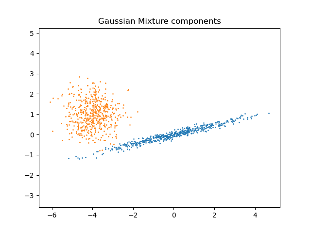
我们通过随机抽样 numpy.random.randn 返回的标准正态分布生成两个组件(每个组件包含 n_samples)。一个组件保持球形,但经过平移和重新缩放。另一个组件变形以具有更通用的协方差矩阵。
import numpy as np

n_samples = 500
np.random.seed(0)
C = np.array([[0.0, -0.1], [1.7, 0.4]])
component_1 = np.dot(np.random.randn(n_samples, 2), C)  # general
component_2 = 0.7 * np.random.randn(n_samples, 2) + np.array([-4, 1])  # spherical

X = np.concatenate([component_1, component_2])
我们可以可视化不同的组件
import matplotlib.pyplot as plt

plt.scatter(component_1[:, 0], component_1[:, 1], s=0.8)
plt.scatter(component_2[:, 0], component_2[:, 1], s=0.8)
plt.title("Gaussian Mixture components")
plt.axis("equal")
plt.show()
模型训练与选择#
我们改变组件数量从 1 到 6 以及要使用的协方差参数类型
"full":每个组件都有自己的通用协方差矩阵。"tied":所有组件共享相同的通用协方差矩阵。"diag":每个组件都有自己的对角协方差矩阵。"spherical":每个组件都有自己的单一方差。
我们对不同的模型进行评分并保留最佳模型(最低的 BIC)。这是通过使用 GridSearchCV 和用户定义的评分函数来实现的,该函数返回负 BIC 分数,因为 GridSearchCV 旨在**最大化**一个分数(最大化负 BIC 等同于最小化 BIC)。
最佳参数集和估计器分别存储在 best_parameters_ 和 best_estimator_ 中。
from sklearn.mixture import GaussianMixture
from sklearn.model_selection import GridSearchCV


def gmm_bic_score(estimator, X):
    """Callable to pass to GridSearchCV that will use the BIC score."""
    # Make it negative since GridSearchCV expects a score to maximize
    return -estimator.bic(X)


param_grid = {
    "n_components": range(1, 7),
    "covariance_type": ["spherical", "tied", "diag", "full"],
}
grid_search = GridSearchCV(
    GaussianMixture(), param_grid=param_grid, scoring=gmm_bic_score
)
grid_search.fit(X)
绘制 BIC 分数#
为了便于绘图,我们可以根据网格搜索的交叉验证结果创建一个 pandas.DataFrame。我们重新反转 BIC 分数的符号,以显示最小化它的效果。
import pandas as pd

df = pd.DataFrame(grid_search.cv_results_)[
    ["param_n_components", "param_covariance_type", "mean_test_score"]
]
df["mean_test_score"] = -df["mean_test_score"]
df = df.rename(
    columns={
        "param_n_components": "Number of components",
        "param_covariance_type": "Type of covariance",
        "mean_test_score": "BIC score",
    }
)
df.sort_values(by="BIC score").head()
import seaborn as sns

sns.catplot(
    data=df,
    kind="bar",
    x="Number of components",
    y="BIC score",
    hue="Type of covariance",
)
plt.show()
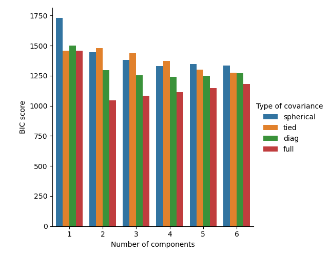
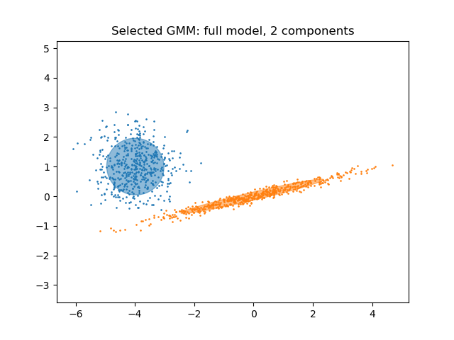
在当前情况下,具有 2 个组件和完整协方差(对应于真实的生成模型)的模型具有最低的 BIC 分数,因此被网格搜索选中。
绘制最佳模型#
我们绘制一个椭圆来显示选定模型的每个高斯分量。为此,需要找到由 covariances_ 属性返回的协方差矩阵的特征值。这些矩阵的形状取决于 covariance_type
"full": (n_components,n_features,n_features)"tied": (n_features,n_features)"diag": (n_components,n_features)"spherical": (n_components,)
from matplotlib.patches import Ellipse
from scipy import linalg

color_iter = sns.color_palette("tab10", 2)[::-1]
Y_ = grid_search.predict(X)

fig, ax = plt.subplots()

for i, (mean, cov, color) in enumerate(
    zip(
        grid_search.best_estimator_.means_,
        grid_search.best_estimator_.covariances_,
        color_iter,
    )
):
    v, w = linalg.eigh(cov)
    if not np.any(Y_ == i):
        continue
    plt.scatter(X[Y_ == i, 0], X[Y_ == i, 1], 0.8, color=color)

    angle = np.arctan2(w[0][1], w[0][0])
    angle = 180.0 * angle / np.pi  # convert to degrees
    v = 2.0 * np.sqrt(2.0) * np.sqrt(v)
    ellipse = Ellipse(mean, v[0], v[1], angle=180.0 + angle, color=color)
    ellipse.set_clip_box(fig.bbox)
    ellipse.set_alpha(0.5)
    ax.add_artist(ellipse)

plt.title(
    f"Selected GMM: {grid_search.best_params_['covariance_type']} model, "
    f"{grid_search.best_params_['n_components']} components"
)
plt.axis("equal")
plt.show()
脚本总运行时间: (0 分钟 1.295 秒)
相关示例