特征缩放的重要性

通过标准化（也称为 Z-score 归一化）进行的特征缩放是许多机器学习算法的重要预处理步骤。它涉及重新缩放每个特征，使其标准差为 1，均值为 0。

尽管基于树的模型（几乎）不受缩放的影响，但许多其他算法要求特征进行归一化，通常出于不同的原因：为了便于收敛（例如非惩罚逻辑回归），为了创建与未缩放数据拟合完全不同的模型拟合（例如 KNeighbors 模型）。后者在本示例的第一部分中得到演示。

在本示例的第二部分中，我们展示了主成分分析 (PCA) 如何受到特征归一化的影响。为了说明这一点，我们比较了使用未缩放数据上的 PCA 找到的主成分与先使用 StandardScaler 缩放数据后获得的主成分。

在示例的最后一部分中，我们展示了归一化对在 PCA 降维数据上训练的模型准确性的影响。

# Authors: The scikit-learn developers
# SPDX-License-Identifier: BSD-3-Clause

加载和准备数据

使用的数据集是 UCI 提供的 葡萄酒识别数据集。该数据集具有连续特征，由于它们测量的属性不同（例如，酒精含量和苹果酸），因此在尺度上存在异构性。

from sklearn.datasets import load_wine
from sklearn.model_selection import train_test_split
from sklearn.preprocessing import StandardScaler

X, y = load_wine(return_X_y=True, as_frame=True)
scaler = StandardScaler().set_output(transform="pandas")

X_train, X_test, y_train, y_test = train_test_split(
    X, y, test_size=0.30, random_state=42
)
scaled_X_train = scaler.fit_transform(X_train)

重新缩放对 k 近邻模型的影响

为了可视化 KNeighborsClassifier 的决策边界，在本节中，我们选择了一个具有不同数量级值的 2 个特征的子集。

请记住，使用特征子集来训练模型可能会遗漏具有高预测影响的特征，从而导致决策边界与在完整特征集上训练的模型相比要差得多。

import matplotlib.pyplot as plt

from sklearn.inspection import DecisionBoundaryDisplay
from sklearn.neighbors import KNeighborsClassifier

X_plot = X[["proline", "hue"]]
X_plot_scaled = scaler.fit_transform(X_plot)
clf = KNeighborsClassifier(n_neighbors=20)


def fit_and_plot_model(X_plot, y, clf, ax):
    clf.fit(X_plot, y)
    disp = DecisionBoundaryDisplay.from_estimator(
        clf,
        X_plot,
        response_method="predict",
        alpha=0.5,
        ax=ax,
    )
    disp.ax_.scatter(X_plot["proline"], X_plot["hue"], c=y, s=20, edgecolor="k")
    disp.ax_.set_xlim((X_plot["proline"].min(), X_plot["proline"].max()))
    disp.ax_.set_ylim((X_plot["hue"].min(), X_plot["hue"].max()))
    return disp.ax_


fig, (ax1, ax2) = plt.subplots(ncols=2, figsize=(12, 6))

fit_and_plot_model(X_plot, y, clf, ax1)
ax1.set_title("KNN without scaling")

fit_and_plot_model(X_plot_scaled, y, clf, ax2)
ax2.set_xlabel("scaled proline")
ax2.set_ylabel("scaled hue")
_ = ax2.set_title("KNN with scaling")

这里的决策边界显示，拟合缩放或未缩放的数据会导致完全不同的模型。原因是变量“proline”的值在 0 到 1,000 之间变化；而变量“hue”的值在 1 到 10 之间变化。因此，样本之间的距离主要受“proline”值的差异影响，而“hue”的值则相对被忽略。如果使用 StandardScaler 对该数据库进行归一化，则两个缩放值都大致在 -3 到 3 之间，并且邻居结构将或多或少地受到两个变量的同等影响。

重新缩放对 PCA 降维的影响

使用 PCA 进行降维包括寻找使方差最大化的特征。如果某个特征的方差比其他特征大，仅仅是因为它们的尺度不同，则 PCA 将确定该特征主导主成分的方向。

我们可以使用所有原始特征来检查第一主成分

import pandas as pd

from sklearn.decomposition import PCA

pca = PCA(n_components=2).fit(X_train)
scaled_pca = PCA(n_components=2).fit(scaled_X_train)
X_train_transformed = pca.transform(X_train)
X_train_std_transformed = scaled_pca.transform(scaled_X_train)

first_pca_component = pd.DataFrame(
    pca.components_[0], index=X.columns, columns=["without scaling"]
)
first_pca_component["with scaling"] = scaled_pca.components_[0]
first_pca_component.plot.bar(
    title="Weights of the first principal component", figsize=(6, 8)
)

_ = plt.tight_layout()

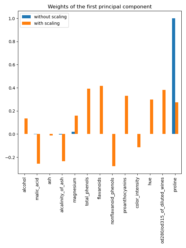
确实，我们发现“proline”特征在没有缩放的情况下主导了第一主成分的方向，比其他特征高出大约两个数量级。这与观察数据的缩放版本的第一主成分形成对比，其中所有特征的数量级大致相同。

我们可以可视化两种情况下的主成分分布

fig, (ax1, ax2) = plt.subplots(nrows=1, ncols=2, figsize=(10, 5))

target_classes = range(0, 3)
colors = ("blue", "red", "green")
markers = ("^", "s", "o")

for target_class, color, marker in zip(target_classes, colors, markers):
    ax1.scatter(
        x=X_train_transformed[y_train == target_class, 0],
        y=X_train_transformed[y_train == target_class, 1],
        color=color,
        label=f"class {target_class}",
        alpha=0.5,
        marker=marker,
    )

    ax2.scatter(
        x=X_train_std_transformed[y_train == target_class, 0],
        y=X_train_std_transformed[y_train == target_class, 1],
        color=color,
        label=f"class {target_class}",
        alpha=0.5,
        marker=marker,
    )

ax1.set_title("Unscaled training dataset after PCA")
ax2.set_title("Standardized training dataset after PCA")

for ax in (ax1, ax2):
    ax.set_xlabel("1st principal component")
    ax.set_ylabel("2nd principal component")
    ax.legend(loc="upper right")
    ax.grid()

_ = plt.tight_layout()

从上面的图中我们观察到，在降维之前缩放特征会使分量具有相同的数量级。在这种情况下，它还提高了类的可分离性。确实，在下一节中，我们确认更好的可分离性对模型的整体性能有很好的影响。

重新缩放对模型性能的影响

首先，我们展示了 LogisticRegressionCV 的最佳正则化如何取决于数据的缩放或未缩放

import numpy as np

from sklearn.linear_model import LogisticRegressionCV
from sklearn.pipeline import make_pipeline

Cs = np.logspace(-5, 5, 20)

unscaled_clf = make_pipeline(
    pca, LogisticRegressionCV(Cs=Cs, use_legacy_attributes=False, l1_ratios=(0,))
)
unscaled_clf.fit(X_train, y_train)

scaled_clf = make_pipeline(
    scaler,
    pca,
    LogisticRegressionCV(Cs=Cs, use_legacy_attributes=False, l1_ratios=(0,)),
)
scaled_clf.fit(X_train, y_train)

print(f"Optimal C for the unscaled PCA: {unscaled_clf[-1].C_:.4f}\n")
print(f"Optimal C for the standardized data with PCA: {scaled_clf[-1].C_:.2f}")

Optimal C for the unscaled PCA: 0.0004

Optimal C for the standardized data with PCA: 20.69

对于未在应用 PCA 之前缩放的数据，对正则化的需求更高（C 值更低）。现在我们评估缩放对最佳模型的准确性和平均对数损失的影响

from sklearn.metrics import accuracy_score, log_loss

y_pred = unscaled_clf.predict(X_test)
y_pred_scaled = scaled_clf.predict(X_test)
y_proba = unscaled_clf.predict_proba(X_test)
y_proba_scaled = scaled_clf.predict_proba(X_test)

print("Test accuracy for the unscaled PCA")
print(f"{accuracy_score(y_test, y_pred):.2%}\n")
print("Test accuracy for the standardized data with PCA")
print(f"{accuracy_score(y_test, y_pred_scaled):.2%}\n")
print("Log-loss for the unscaled PCA")
print(f"{log_loss(y_test, y_proba):.3}\n")
print("Log-loss for the standardized data with PCA")
print(f"{log_loss(y_test, y_proba_scaled):.3}")

Test accuracy for the unscaled PCA
35.19%

Test accuracy for the standardized data with PCA
96.30%

Log-loss for the unscaled PCA
0.957

Log-loss for the standardized data with PCA
0.0825

当在 PCA 之前缩放数据时，预测准确性有明显的差异，因为它大大优于未缩放的版本。这与从上一节的图中获得的直觉相对应，其中在使用 PCA 之前进行缩放时，分量变得线性可分。

请注意，在这种情况下，具有缩放特征的模型比具有非缩放特征的模型表现更好，因为所有变量都被认为是具有预测性的，我们宁愿避免其中一些变量被相对忽略。

如果尺度较低的变量不具有预测性，则在缩放特征后可能会遇到性能下降：缩放后，嘈杂特征对预测的贡献会更大，因此缩放会增加过拟合。

最后但同样重要的是，我们观察到通过缩放步骤可以实现更低的对数损失。

相关示例

SVC 的正则化参数缩放

SVC 的正则化参数缩放

比较线性贝叶斯回归器

比较线性贝叶斯回归器

核 PCA

核 PCA

最近邻分类

最近邻分类