F-test和互信息比较#

此示例说明了单变量F-test统计量和互信息之间的差异。

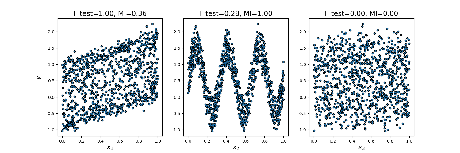
我们考虑3个特征x_1, x_2, x_3，它们均匀分布在[0, 1]上，目标y与它们的关系如下：

y = x_1 + sin(6 * pi * x_2) + 0.1 * N(0, 1)，即第三个特征完全不相关。

下面的代码绘制了y与单个x_i的依赖关系，以及单变量F-test统计量和互信息的归一化值。

由于F-test仅捕获线性依赖关系，它将x_1评为最具区分度的特征。另一方面，互信息可以捕获变量之间任何类型的依赖关系，它将x_2评为最具区分度的特征，这可能与我们对这个示例的直观感知更一致。两种方法都正确地将x_3标记为不相关。

F-test=1.00, MI=0.36, F-test=0.28, MI=1.00, F-test=0.00, MI=0.00

# Authors: The scikit-learn developers
# SPDX-License-Identifier: BSD-3-Clause

import matplotlib.pyplot as plt
import numpy as np

from sklearn.feature_selection import f_regression, mutual_info_regression

np.random.seed(0)
X = np.random.rand(1000, 3)
y = X[:, 0] + np.sin(6 * np.pi * X[:, 1]) + 0.1 * np.random.randn(1000)

f_test, _ = f_regression(X, y)
f_test /= np.max(f_test)

mi = mutual_info_regression(X, y)
mi /= np.max(mi)

plt.figure(figsize=(15, 5))
for i in range(3):
    plt.subplot(1, 3, i + 1)
    plt.scatter(X[:, i], y, edgecolor="black", s=20)
    plt.xlabel("$x_{}$".format(i + 1), fontsize=14)
    if i == 0:
        plt.ylabel("$y$", fontsize=14)
    plt.title("F-test={:.2f}, MI={:.2f}".format(f_test[i], mi[i]), fontsize=16)
plt.show()

脚本总运行时间： (0 minutes 0.184 seconds)

F-test和互信息比较#

本页