注意
转到末尾以下载完整示例代码,或通过 JupyterLite 或 Binder 在浏览器中运行此示例。
梯度提升中的分类特征支持#
在此示例中,我们比较了 HistGradientBoostingRegressor 在不同分类特征编码策略下的训练时间和预测性能。具体来说,我们评估了以下策略:
“Dropped”(丢弃):丢弃分类特征;
“One Hot”(独热编码):使用
OneHotEncoder;“Ordinal”(序数编码):使用
OrdinalEncoder并将类别视为有序、等距的量;“Target”(目标编码):使用
TargetEncoder;“Native”(原生支持):依赖
HistGradientBoostingRegressor估计器的原生类别支持。
为此,我们使用 Ames Iowa Housing 数据集,该数据集包含数值和分类特征,目标是房屋销售价格。
有关 HistGradientBoostingRegressor 其他功能示例,请参阅直方图梯度提升树中的特征。
有关高基数分类特征存在时的编码策略比较,请参阅目标编码器与其他编码器的比较。
# Authors: The scikit-learn developers
# SPDX-License-Identifier: BSD-3-Clause
加载 Ames Housing 数据集#
首先,我们将 Ames Housing 数据作为 pandas 数据帧加载。特征要么是分类的,要么是数值的。
from sklearn.datasets import fetch_openml

X, y = fetch_openml(data_id=42165, as_frame=True, return_X_y=True)

# Select only a subset of features of X to make the example faster to run
categorical_columns_subset = [
    "BldgType",
    "GarageFinish",
    "LotConfig",
    "Functional",
    "MasVnrType",
    "HouseStyle",
    "FireplaceQu",
    "ExterCond",
    "ExterQual",
    "PoolQC",
]

numerical_columns_subset = [
    "3SsnPorch",
    "Fireplaces",
    "BsmtHalfBath",
    "HalfBath",
    "GarageCars",
    "TotRmsAbvGrd",
    "BsmtFinSF1",
    "BsmtFinSF2",
    "GrLivArea",
    "ScreenPorch",
]

X = X[categorical_columns_subset + numerical_columns_subset]
X[categorical_columns_subset] = X[categorical_columns_subset].astype("category")

categorical_columns = X.select_dtypes(include="category").columns
n_categorical_features = len(categorical_columns)
n_numerical_features = X.select_dtypes(include="number").shape[1]

print(f"Number of samples: {X.shape[0]}")
print(f"Number of features: {X.shape[1]}")
print(f"Number of categorical features: {n_categorical_features}")
print(f"Number of numerical features: {n_numerical_features}")
Number of samples: 1460
Number of features: 20
Number of categorical features: 10
Number of numerical features: 10
丢弃分类特征的梯度提升估计器#
作为基线,我们创建一个丢弃分类特征的估计器。
from sklearn.compose import make_column_selector, make_column_transformer
from sklearn.ensemble import HistGradientBoostingRegressor
from sklearn.pipeline import make_pipeline

dropper = make_column_transformer(
    ("drop", make_column_selector(dtype_include="category")), remainder="passthrough"
)
hist_dropped = make_pipeline(dropper, HistGradientBoostingRegressor(random_state=42))
hist_dropped
Pipeline(steps=[('columntransformer',
                 ColumnTransformer(remainder='passthrough',
                                   transformers=[('drop', 'drop',
                                                  <sklearn.compose._column_transformer.make_column_selector object at 0x7fb4a2b293d0>)])),
                ('histgradientboostingregressor',
                 HistGradientBoostingRegressor(random_state=42))])
在 Jupyter 环境中,请重新运行此单元格以显示 HTML 表示形式或信任 notebook。在 GitHub 上,HTML 表示形式无法渲染,请尝试使用 nbviewer.org 加载此页面。
参数
参数
<sklearn.compose._column_transformer.make_column_selector object at 0x7fb4a2b293d0>
drop
passthrough
参数
使用独热编码的梯度提升估计器#
接下来,我们创建一个流水线,用于对分类特征进行独热编码,同时让其余特征 "passthrough" 保持不变。
from sklearn.preprocessing import OneHotEncoder

one_hot_encoder = make_column_transformer(
    (
        OneHotEncoder(sparse_output=False, handle_unknown="ignore"),
        make_column_selector(dtype_include="category"),
    ),
    remainder="passthrough",
)

hist_one_hot = make_pipeline(
    one_hot_encoder, HistGradientBoostingRegressor(random_state=42)
)
hist_one_hot
Pipeline(steps=[('columntransformer',
                 ColumnTransformer(remainder='passthrough',
                                   transformers=[('onehotencoder',
                                                  OneHotEncoder(handle_unknown='ignore',
                                                                sparse_output=False),
                                                  <sklearn.compose._column_transformer.make_column_selector object at 0x7fb4a2b28f50>)])),
                ('histgradientboostingregressor',
                 HistGradientBoostingRegressor(random_state=42))])
在 Jupyter 环境中,请重新运行此单元格以显示 HTML 表示形式或信任 notebook。在 GitHub 上,HTML 表示形式无法渲染,请尝试使用 nbviewer.org 加载此页面。
参数
参数
<sklearn.compose._column_transformer.make_column_selector object at 0x7fb4a2b28f50>
参数
passthrough
参数
使用序数编码的梯度提升估计器#
接下来,我们创建一个流水线,将分类特征视为有序数量,即类别被编码为 0、1、2 等,并被视为连续特征。
import numpy as np

from sklearn.preprocessing import OrdinalEncoder

ordinal_encoder = make_column_transformer(
    (
        OrdinalEncoder(handle_unknown="use_encoded_value", unknown_value=np.nan),
        make_column_selector(dtype_include="category"),
    ),
    remainder="passthrough",
)

hist_ordinal = make_pipeline(
    ordinal_encoder, HistGradientBoostingRegressor(random_state=42)
)
hist_ordinal
Pipeline(steps=[('columntransformer',
                 ColumnTransformer(remainder='passthrough',
                                   transformers=[('ordinalencoder',
                                                  OrdinalEncoder(handle_unknown='use_encoded_value',
                                                                 unknown_value=nan),
                                                  <sklearn.compose._column_transformer.make_column_selector object at 0x7fb4a1b6f790>)])),
                ('histgradientboostingregressor',
                 HistGradientBoostingRegressor(random_state=42))])
在 Jupyter 环境中,请重新运行此单元格以显示 HTML 表示形式或信任 notebook。在 GitHub 上,HTML 表示形式无法渲染,请尝试使用 nbviewer.org 加载此页面。
参数
参数
<sklearn.compose._column_transformer.make_column_selector object at 0x7fb4a1b6f790>
参数
passthrough
参数
使用目标编码的梯度提升估计器#
另一种可能性是使用 TargetEncoder,它根据平滑的 np.mean(y, axis=0) 计算的(训练)目标变量的均值来编码类别,即:
在回归中,它使用
y的均值;在二元分类中,使用正类率;
在多类别分类中,使用类别率向量(每个类别一个)。
对于每个类别,它使用交叉拟合计算这些目标平均值,这意味着训练数据被分成几折:在每一折中,平均值仅在数据子集上计算,然后应用于保留部分。这样,每个样本都使用它未参与的数据中的统计信息进行编码,从而防止目标信息泄露。
from sklearn.preprocessing import TargetEncoder

target_encoder = make_column_transformer(
    (
        TargetEncoder(target_type="continuous", random_state=42),
        make_column_selector(dtype_include="category"),
    ),
    remainder="passthrough",
)

hist_target = make_pipeline(
    target_encoder, HistGradientBoostingRegressor(random_state=42)
)
hist_target
Pipeline(steps=[('columntransformer',
                 ColumnTransformer(remainder='passthrough',
                                   transformers=[('targetencoder',
                                                  TargetEncoder(random_state=42,
                                                                target_type='continuous'),
                                                  <sklearn.compose._column_transformer.make_column_selector object at 0x7fb4a1b6f2d0>)])),
                ('histgradientboostingregressor',
                 HistGradientBoostingRegressor(random_state=42))])
在 Jupyter 环境中,请重新运行此单元格以显示 HTML 表示形式或信任 notebook。在 GitHub 上,HTML 表示形式无法渲染,请尝试使用 nbviewer.org 加载此页面。
参数
参数
<sklearn.compose._column_transformer.make_column_selector object at 0x7fb4a1b6f2d0>
参数
passthrough
参数
具有原生分类支持的梯度提升估计器#
现在我们创建一个 HistGradientBoostingRegressor 估计器,它可以原生处理分类特征而无需显式编码。通过设置 categorical_features="from_dtype"(自动检测具有分类 dtypes 的特征),或者更明确地通过 categorical_features=categorical_columns_subset 来启用此功能。
与之前的编码方法不同,估计器原生处理分类特征。在每次拆分时,它使用一种启发式方法将此类特征的类别划分为不相交的集合,该方法根据类别对目标变量的影响对它们进行排序,详情请参阅 Split finding with categorical features。
虽然序数编码对于低基数特征可能效果很好,即使类别没有自然顺序,但随着基数增加,实现有意义的拆分需要更深的树。原生分类支持通过直接处理无序类别来避免这种情况。与独热编码相比,优点是省略了预处理,并且拟合和预测时间更快。
hist_native = HistGradientBoostingRegressor(
    random_state=42, categorical_features="from_dtype"
)
hist_native
HistGradientBoostingRegressor(random_state=42)在 Jupyter 环境中,请重新运行此单元格以显示 HTML 表示形式或信任 notebook。
在 GitHub 上,HTML 表示形式无法渲染,请尝试使用 nbviewer.org 加载此页面。
参数
模型比较#
在这里,我们使用交叉验证来比较模型在 mean_absolute_percentage_error 方面的性能和拟合时间。在即将出现的图中,误差条代表通过交叉验证拆分计算出的 1 个标准差。
from sklearn.model_selection import cross_validate

common_params = {"cv": 5, "scoring": "neg_mean_absolute_percentage_error", "n_jobs": -1}

dropped_result = cross_validate(hist_dropped, X, y, **common_params)
one_hot_result = cross_validate(hist_one_hot, X, y, **common_params)
ordinal_result = cross_validate(hist_ordinal, X, y, **common_params)
target_result = cross_validate(hist_target, X, y, **common_params)
native_result = cross_validate(hist_native, X, y, **common_params)
results = [
    ("Dropped", dropped_result),
    ("One Hot", one_hot_result),
    ("Ordinal", ordinal_result),
    ("Target", target_result),
    ("Native", native_result),
]
import matplotlib.pyplot as plt
import matplotlib.ticker as ticker


def plot_performance_tradeoff(results, title):
    fig, ax = plt.subplots()
    markers = ["s", "o", "^", "x", "D"]

    for idx, (name, result) in enumerate(results):
        test_error = -result["test_score"]
        mean_fit_time = np.mean(result["fit_time"])
        mean_score = np.mean(test_error)
        std_fit_time = np.std(result["fit_time"])
        std_score = np.std(test_error)

        ax.scatter(
            result["fit_time"],
            test_error,
            label=name,
            marker=markers[idx],
        )
        ax.scatter(
            mean_fit_time,
            mean_score,
            color="k",
            marker=markers[idx],
        )
        ax.errorbar(
            x=mean_fit_time,
            y=mean_score,
            yerr=std_score,
            c="k",
            capsize=2,
        )
        ax.errorbar(
            x=mean_fit_time,
            y=mean_score,
            xerr=std_fit_time,
            c="k",
            capsize=2,
        )

    ax.set_xscale("log")

    nticks = 7
    x0, x1 = np.log10(ax.get_xlim())
    ticks = np.logspace(x0, x1, nticks)
    ax.set_xticks(ticks)
    ax.xaxis.set_major_formatter(ticker.FormatStrFormatter("%1.1e"))
    ax.minorticks_off()

    ax.annotate(
        "  best\nmodels",
        xy=(0.04, 0.04),
        xycoords="axes fraction",
        xytext=(0.09, 0.14),
        textcoords="axes fraction",
        arrowprops=dict(arrowstyle="->", lw=1.5),
    )
    ax.set_xlabel("Time to fit (seconds)")
    ax.set_ylabel("Mean Absolute Percentage Error")
    ax.set_title(title)
    ax.legend()
    plt.show()


plot_performance_tradeoff(results, "Gradient Boosting on Ames Housing")

在上面的图中,"最佳模型"是那些更接近左下角的模型,如箭头所示。这些模型将对应于更快的拟合和更低的误差。
使用独热编码数据的模型最慢。这是可以预料到的,因为独热编码会为每个分类特征的每个类别值创建一个额外的特征,从而大大增加训练期间的拆分候选数量。理论上,我们预计原生处理分类特征会比将类别视为有序数量(“Ordinal”)略慢,因为原生处理需要对类别进行排序。然而,当类别数量较少时,拟合时间应该接近,但这在实践中可能并不总是得到体现。
使用 TargetEncoder 进行拟合所需的时间取决于交叉拟合参数 cv,因为增加拆分会带来计算成本。
在预测性能方面,丢弃分类特征会导致最差的性能。利用分类特征的四个模型具有可比的错误率,其中原生处理略有优势。
限制拆分次数#
通常,可以预期独热编码数据的预测效果较差,尤其是当树深或节点数受限时:对于独热编码数据,需要更多的拆分点,即更深的深度,才能恢复在原生处理中可以在一个拆分点获得的等效拆分。
当类别被视为序数量时也是如此:如果类别是 A..F 且最佳拆分是 ACF - BDE,则独热编码模型需要 3 个拆分点(左节点中每个类别一个),而序数非原生模型需要 4 个拆分:1 个拆分隔离 A,1 个拆分隔离 F,以及 2 个拆分隔离 C 和 BCDE。
模型性能在实践中差异的强度取决于数据集和树的灵活性。
为了说明这一点,让我们在欠拟合模型中重新运行相同的分析,其中我们通过限制树的数量和每棵树的深度来人为地限制总拆分次数。
for pipe in (hist_dropped, hist_one_hot, hist_ordinal, hist_target, hist_native):
    if pipe is hist_native:
        # The native model does not use a pipeline so, we can set the parameters
        # directly.
        pipe.set_params(max_depth=3, max_iter=15)
    else:
        pipe.set_params(
            histgradientboostingregressor__max_depth=3,
            histgradientboostingregressor__max_iter=15,
        )

dropped_result = cross_validate(hist_dropped, X, y, **common_params)
one_hot_result = cross_validate(hist_one_hot, X, y, **common_params)
ordinal_result = cross_validate(hist_ordinal, X, y, **common_params)
target_result = cross_validate(hist_target, X, y, **common_params)
native_result = cross_validate(hist_native, X, y, **common_params)
results_underfit = [
    ("Dropped", dropped_result),
    ("One Hot", one_hot_result),
    ("Ordinal", ordinal_result),
    ("Target", target_result),
    ("Native", native_result),
]
plot_performance_tradeoff(
    results_underfit, "Gradient Boosting on Ames Housing (few and shallow trees)"
)
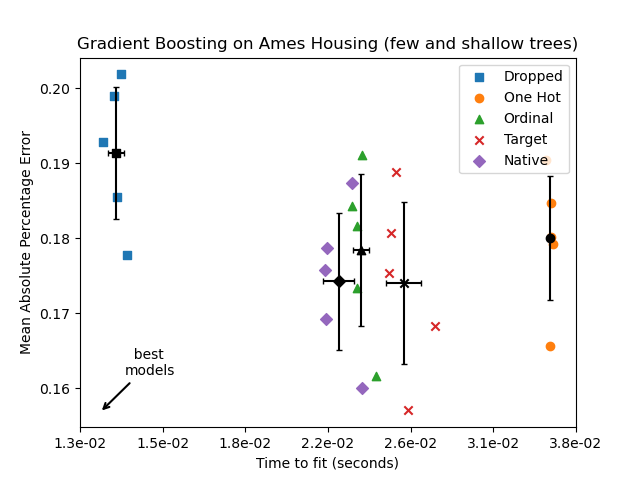
这些欠拟合模型的结果证实了我们先前的直觉:当拆分预算受限时,原生类别处理策略表现最佳。三种显式编码策略(独热编码、序数编码和目标编码)导致的误差略大于估计器的原生处理,但仍优于完全丢弃分类特征的基线模型。
脚本总运行时间: (0 minutes 4.379 seconds)
相关示例