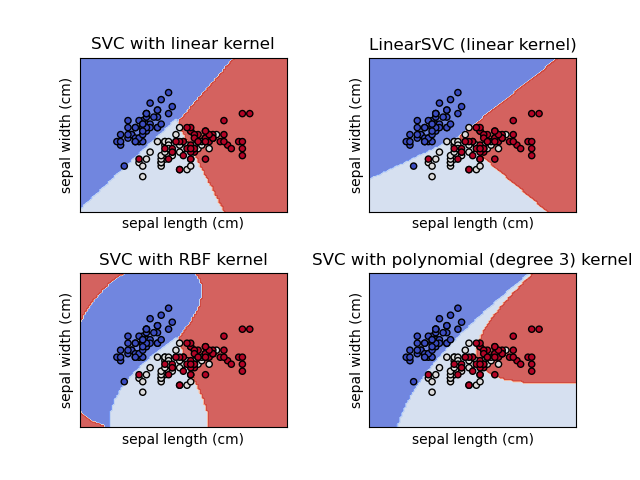
在鸢尾花数据集上绘制不同的SVM分类器#

在鸢尾花数据集的2D投影上比较不同的线性SVM分类器。我们只考虑此数据集的前2个特征

萼片长度
萼片宽度

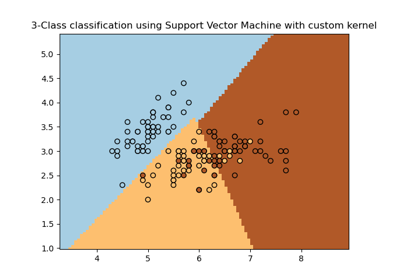
此示例演示如何绘制具有不同核的四个SVM分类器的决策面。

线性模型 LinearSVC() 和 SVC(kernel='linear') 会产生略微不同的决策边界。这可能是由于以下差异造成的：

LinearSVC 最小化平方合页损失（squared hinge loss），而 SVC 最小化正则合页损失（regular hinge loss）。
LinearSVC 使用“一对多”（One-vs-All，也称为One-vs-Rest）多类别归约，而 SVC 使用“一对一”（One-vs-One）多类别归约。

两种线性模型都具有线性决策边界（相交的超平面），而非线性核模型（多项式或高斯RBF）具有更灵活的非线性决策边界，其形状取决于核的类型及其参数。

注意

虽然为玩具2D数据集绘制分类器的决策函数有助于直观理解它们各自的表达能力，但请注意，这些直觉并不总是能推广到更现实的高维问题。

SVC with linear kernel, LinearSVC (linear kernel), SVC with RBF kernel, SVC with polynomial (degree 3) kernel

# Authors: The scikit-learn developers
# SPDX-License-Identifier: BSD-3-Clause

import matplotlib.pyplot as plt

from sklearn import datasets, svm
from sklearn.inspection import DecisionBoundaryDisplay

# import some data to play with
iris = datasets.load_iris()
# Take the first two features. We could avoid this by using a two-dim dataset
X = iris.data[:, :2]
y = iris.target

# we create an instance of SVM and fit out data. We do not scale our
# data since we want to plot the support vectors
C = 1.0  # SVM regularization parameter
models = (
    svm.SVC(kernel="linear", C=C),
    svm.LinearSVC(C=C, max_iter=10000),
    svm.SVC(kernel="rbf", gamma=0.7, C=C),
    svm.SVC(kernel="poly", degree=3, gamma="auto", C=C),
)
models = (clf.fit(X, y) for clf in models)

# title for the plots
titles = (
    "SVC with linear kernel",
    "LinearSVC (linear kernel)",
    "SVC with RBF kernel",
    "SVC with polynomial (degree 3) kernel",
)

# Set-up 2x2 grid for plotting.
fig, sub = plt.subplots(2, 2)
plt.subplots_adjust(wspace=0.4, hspace=0.4)

X0, X1 = X[:, 0], X[:, 1]

for clf, title, ax in zip(models, titles, sub.flatten()):
    disp = DecisionBoundaryDisplay.from_estimator(
        clf,
        X,
        response_method="predict",
        cmap=plt.cm.coolwarm,
        alpha=0.8,
        ax=ax,
        xlabel=iris.feature_names[0],
        ylabel=iris.feature_names[1],
    )
    ax.scatter(X0, X1, c=y, cmap=plt.cm.coolwarm, s=20, edgecolors="k")
    ax.set_xticks(())
    ax.set_yticks(())
    ax.set_title(title)

plt.show()

脚本总运行时间： (0 minutes 0.166 seconds)

在鸢尾花数据集上绘制不同的SVM分类器#

本页