使用混淆矩阵评估分类器性能#

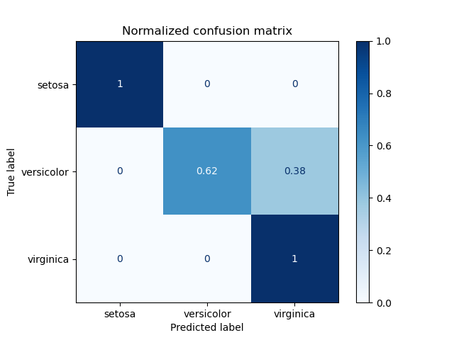
使用混淆矩阵评估鸢尾花数据集上分类器输出质量的示例。对角线元素表示预测标签等于真实标签的点数，而非对角线元素则表示被分类器错误标记的点。混淆矩阵的对角线值越高越好，表明有许多正确的预测。

这些图显示了混淆矩阵，包括按类别支持大小（每个类别中的元素数量）进行标准化和不进行标准化的两种情况。这种标准化在类别不平衡的情况下会很有用，可以更直观地解释哪个类别被错误分类了。

这里的结果不如预期的好，因为我们对正则化参数 C 的选择不是最佳的。在实际应用中，这个参数通常使用调整估计器的超参数来选择。

# Authors: The scikit-learn developers
# SPDX-License-Identifier: BSD-3-Clause

import matplotlib.pyplot as plt
import numpy as np

from sklearn import datasets, svm
from sklearn.metrics import ConfusionMatrixDisplay
from sklearn.model_selection import train_test_split

# import some data to play with
iris = datasets.load_iris()
X = iris.data
y = iris.target
class_names = iris.target_names

# Split the data into a training set and a test set
X_train, X_test, y_train, y_test = train_test_split(X, y, random_state=0)

# Run classifier, using a model that is too regularized (C too low) to see
# the impact on the results
classifier = svm.SVC(kernel="linear", C=0.01).fit(X_train, y_train)

np.set_printoptions(precision=2)

# Plot non-normalized confusion matrix
titles_options = [
    ("Confusion matrix, without normalization", None),
    ("Normalized confusion matrix", "true"),
]
for title, normalize in titles_options:
    disp = ConfusionMatrixDisplay.from_estimator(
        classifier,
        X_test,
        y_test,
        display_labels=class_names,
        cmap=plt.cm.Blues,
        normalize=normalize,
    )
    disp.ax_.set_title(title)

    print(title)
    print(disp.confusion_matrix)

plt.show()

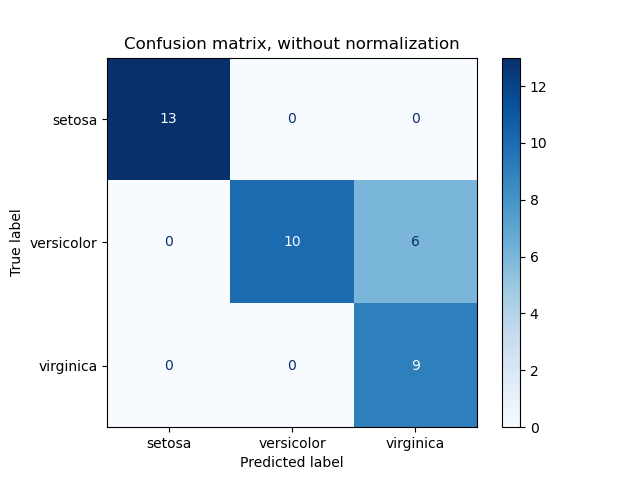
Confusion matrix, without normalization
[[13  0  0]
 [ 0 10  6]
 [ 0  0  9]]
Normalized confusion matrix
[[1.   0.   0.  ]
 [0.   0.62 0.38]
 [0.   0.   1.  ]]

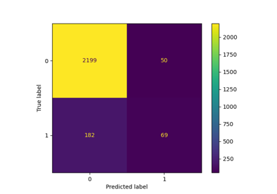
二元分类#

对于二元问题，sklearn.metrics.confusion_matrix有一个ravel方法，我们可以用来获取真负例、假正例、假负例和真正例的计数。

要在不同阈值下获取真负例、假正例、假负例和真正例的计数，可以使用sklearn.metrics.confusion_matrix_at_thresholds。这对于二元分类指标（如roc_auc_score和det_curve）至关重要。

from sklearn.datasets import make_classification
from sklearn.metrics import confusion_matrix_at_thresholds

X, y = make_classification(
    n_samples=100,
    n_features=20,
    n_informative=20,
    n_redundant=0,
    n_classes=2,
    random_state=42,
)

X_train, X_test, y_train, y_test = train_test_split(
    X, y, test_size=0.3, random_state=42
)

classifier = svm.SVC(kernel="linear", C=0.01, probability=True)
classifier.fit(X_train, y_train)

y_score = classifier.predict_proba(X_test)[:, 1]

tns, fps, fns, tps, threshold = confusion_matrix_at_thresholds(y_test, y_score)

# Plot TNs, FPs, FNs and TPs vs Thresholds
plt.figure(figsize=(10, 6))

plt.plot(threshold, tns, label="True Negatives (TNs)")
plt.plot(threshold, fps, label="False Positives (FPs)")
plt.plot(threshold, fns, label="False Negatives (FNs)")
plt.plot(threshold, tps, label="True Positives (TPs)")
plt.xlabel("Thresholds")
plt.ylabel("Count")
plt.title("TNs, FPs, FNs and TPs vs Thresholds")
plt.legend()
plt.grid()

plt.show()

脚本总运行时间： (0 分钟 0.243 秒)

使用混淆矩阵评估分类器性能#

二元分类#

本页