稳健的协方差估计和马哈拉诺比斯距离的相关性#

此示例展示了使用马哈拉诺比斯距离对高斯分布数据进行协方差估计。

对于高斯分布数据，观测值 \(x_i\) 到分布众数的距离可以使用其马哈拉诺比斯距离计算：

\[d_{(\mu,\Sigma)}(x_i)^2 = (x_i - \mu)^T\Sigma^{-1}(x_i - \mu)\]

其中 \(\mu\) 和 \(\Sigma\) 是底层高斯分布的位置和协方差。

在实践中，\(\mu\) 和 \(\Sigma\) 被替换为一些估计值。标准的协方差最大似然估计（MLE）对数据集中离群值的存在非常敏感，因此，下游的马哈拉诺比斯距离也如此。最好使用稳健的协方差估计器来确保估计值能抵抗数据集中的“错误”观测值，并且计算出的马哈拉诺比斯距离能准确反映观测值的真实组织结构。

最小协方差行列式估计器（MCD）是一种稳健的、高击穿点（即它可用于估计高度受污染数据集的协方差矩阵，击穿点高达 \(\frac{n_\text{samples}-n_\text{features}-1}{2}\) 个离群值）的协方差估计器。MCD背后的思想是找到 \(\frac{n_\text{samples}+n_\text{features}+1}{2}\) 个经验协方差具有最小行列式的观测值，从而产生一个“纯净”的观测值子集，并从中计算标准的位置和协方差估计值。MCD由P.J.Rousseuw在[1]中引入。

此示例说明了马哈拉诺比斯距离如何受到离群数据的影响。当使用基于标准协方差MLE的马哈拉诺比斯距离时，从污染分布中提取的观测值无法与来自真实高斯分布的观测值区分开来。使用基于MCD的马哈拉诺比斯距离，这两个群体变得可区分。相关的应用包括离群值检测、观测值排名和聚类。

注意

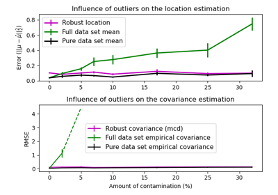
另请参阅稳健协方差估计与经验协方差估计的比较

References

# Authors: The scikit-learn developers
# SPDX-License-Identifier: BSD-3-Clause

生成数据#

首先，我们生成一个包含125个样本和2个特征的数据集。两个特征都呈均值为0的高斯分布，但特征1的标准差等于2，特征2的标准差等于1。接下来，25个样本被替换为高斯离群值样本，其中特征1的标准差等于1，特征2的标准差等于7。

import numpy as np

# for consistent results
np.random.seed(7)

n_samples = 125
n_outliers = 25
n_features = 2

# generate Gaussian data of shape (125, 2)
gen_cov = np.eye(n_features)
gen_cov[0, 0] = 2.0
X = np.dot(np.random.randn(n_samples, n_features), gen_cov)
# add some outliers
outliers_cov = np.eye(n_features)
outliers_cov[np.arange(1, n_features), np.arange(1, n_features)] = 7.0
X[-n_outliers:] = np.dot(np.random.randn(n_outliers, n_features), outliers_cov)

结果比较#

下面，我们将基于MCD和MLE的协方差估计器拟合到我们的数据中，并打印估计的协方差矩阵。请注意，基于MLE的估计器（7.5）估计的特征2方差远高于基于MCD的稳健估计器（1.2）。这表明基于MCD的稳健估计器对离群值样本更具抵抗力，这些离群值样本被设计成在特征2中具有更大的方差。

import matplotlib.pyplot as plt

from sklearn.covariance import EmpiricalCovariance, MinCovDet

# fit a MCD robust estimator to data
robust_cov = MinCovDet().fit(X)
# fit a MLE estimator to data
emp_cov = EmpiricalCovariance().fit(X)
print(
    "Estimated covariance matrix:\nMCD (Robust):\n{}\nMLE:\n{}".format(
        robust_cov.covariance_, emp_cov.covariance_
    )
)

Estimated covariance matrix:
MCD (Robust):
[[ 3.60075119 -0.07640781]
 [-0.07640781  1.51855963]]
MLE:
[[ 3.23773583 -0.24640578]
 [-0.24640578  7.51963999]]

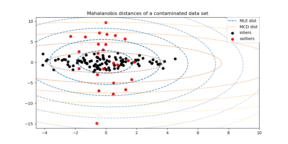
为了更好地可视化差异，我们绘制了两种方法计算的马哈拉诺比斯距离等高线。请注意，基于MCD的稳健马哈拉诺比斯距离更好地拟合了内点（黑色点），而基于MLE的距离则受离群值（红色点）的影响更大。

import matplotlib.lines as mlines

fig, ax = plt.subplots(figsize=(10, 5))
# Plot data set
inlier_plot = ax.scatter(X[:, 0], X[:, 1], color="black", label="inliers")
outlier_plot = ax.scatter(
    X[:, 0][-n_outliers:], X[:, 1][-n_outliers:], color="red", label="outliers"
)
ax.set_xlim(ax.get_xlim()[0], 10.0)
ax.set_title("Mahalanobis distances of a contaminated data set")

# Create meshgrid of feature 1 and feature 2 values
xx, yy = np.meshgrid(
    np.linspace(plt.xlim()[0], plt.xlim()[1], 100),
    np.linspace(plt.ylim()[0], plt.ylim()[1], 100),
)
zz = np.c_[xx.ravel(), yy.ravel()]
# Calculate the MLE based Mahalanobis distances of the meshgrid
mahal_emp_cov = emp_cov.mahalanobis(zz)
mahal_emp_cov = mahal_emp_cov.reshape(xx.shape)
emp_cov_contour = plt.contour(
    xx, yy, np.sqrt(mahal_emp_cov), cmap=plt.cm.PuBu_r, linestyles="dashed"
)
# Calculate the MCD based Mahalanobis distances
mahal_robust_cov = robust_cov.mahalanobis(zz)
mahal_robust_cov = mahal_robust_cov.reshape(xx.shape)
robust_contour = ax.contour(
    xx, yy, np.sqrt(mahal_robust_cov), cmap=plt.cm.YlOrBr_r, linestyles="dotted"
)

# Add legend
ax.legend(
    [
        mlines.Line2D([], [], color="tab:blue", linestyle="dashed"),
        mlines.Line2D([], [], color="tab:orange", linestyle="dotted"),
        inlier_plot,
        outlier_plot,
    ],
    ["MLE dist", "MCD dist", "inliers", "outliers"],
    loc="upper right",
    borderaxespad=0,
)

plt.show()

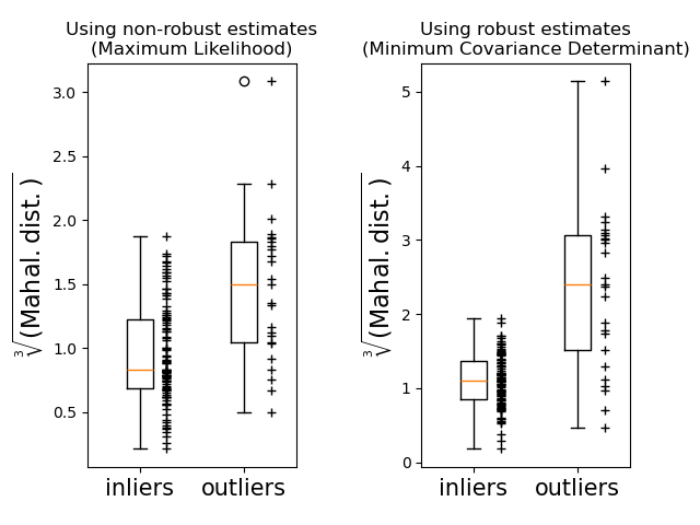
Mahalanobis distances of a contaminated data set

最后，我们强调了基于MCD的马哈拉诺比斯距离区分离群值的能力。我们取马哈拉诺比斯距离的立方根，得到近似正态分布（如Wilson和Hilferty所建议的[2]），然后用箱线图绘制内点和离群值样本的值。对于基于MCD的稳健马哈拉诺比斯距离，离群值样本的分布与内点样本的分布分离得更开。

fig, (ax1, ax2) = plt.subplots(1, 2)
plt.subplots_adjust(wspace=0.6)

# Calculate cubic root of MLE Mahalanobis distances for samples
emp_mahal = emp_cov.mahalanobis(X - np.mean(X, 0)) ** (0.33)
# Plot boxplots
ax1.boxplot([emp_mahal[:-n_outliers], emp_mahal[-n_outliers:]], widths=0.25)
# Plot individual samples
ax1.plot(
    np.full(n_samples - n_outliers, 1.26),
    emp_mahal[:-n_outliers],
    "+k",
    markeredgewidth=1,
)
ax1.plot(np.full(n_outliers, 2.26), emp_mahal[-n_outliers:], "+k", markeredgewidth=1)
ax1.axes.set_xticklabels(("inliers", "outliers"), size=15)
ax1.set_ylabel(r"$\sqrt[3]{\rm{(Mahal. dist.)}}$", size=16)
ax1.set_title("Using non-robust estimates\n(Maximum Likelihood)")

# Calculate cubic root of MCD Mahalanobis distances for samples
robust_mahal = robust_cov.mahalanobis(X - robust_cov.location_) ** (0.33)
# Plot boxplots
ax2.boxplot([robust_mahal[:-n_outliers], robust_mahal[-n_outliers:]], widths=0.25)
# Plot individual samples
ax2.plot(
    np.full(n_samples - n_outliers, 1.26),
    robust_mahal[:-n_outliers],
    "+k",
    markeredgewidth=1,
)
ax2.plot(np.full(n_outliers, 2.26), robust_mahal[-n_outliers:], "+k", markeredgewidth=1)
ax2.axes.set_xticklabels(("inliers", "outliers"), size=15)
ax2.set_ylabel(r"$\sqrt[3]{\rm{(Mahal. dist.)}}$", size=16)
ax2.set_title("Using robust estimates\n(Minimum Covariance Determinant)")

plt.show()

Using non-robust estimates (Maximum Likelihood), Using robust estimates (Minimum Covariance Determinant)

脚本总运行时间： (0 minutes 0.228 seconds)

稳健的协方差估计和马哈拉诺比斯距离的相关性#

生成数据#

结果比较#

本页