注意
转至末尾以下载完整示例代码或通过 JupyterLite 或 Binder 在浏览器中运行此示例。
Precision-Recall(精确度-召回率)#
用于评估分类器输出质量的 Precision-Recall(精确度-召回率)指标示例。
当类别非常不平衡时,精确度-召回率是衡量预测成功与否的有用指标。在信息检索中,精确度衡量的是实际返回的项目中相关项目的比例,而召回率衡量的是在所有应该返回的项目中已返回的项目的比例。“相关性”在这里指的是被标记为正例的项目,即真阳性(true positives)和假阴性(false negatives)。
精确度(\(P\))定义为真阳性(\(T_p\))的数量除以真阳性数量加上假阳性(\(F_p\))数量。
召回率(\(R\))定义为真阳性(\(T_p\))的数量除以真阳性数量加上假阴性(\(F_n\))数量。
精确度-召回率曲线显示了不同阈值下精确度和召回率之间的权衡。曲线下的高面积代表高召回率和高精确度。高精确度是通过在返回结果中包含少量假阳性来实现的,而高召回率是通过在相关结果中包含少量假阴性来实现的。两者都得分高表明分类器返回的结果准确(高精确度),并且返回了大多数相关结果(高召回率)。
具有高召回率但低精确度的系统会返回大多数相关项目,但返回结果中被错误标记的比例很高。具有高精确度但低召回率的系统则恰好相反,它返回的相关项目非常少,但其预测的大多数标签与实际标签相比是正确的。具有高精确度和高召回率的理想系统将返回大多数相关项目,且大多数结果被正确标记。
精确度的定义(\(\frac{T_p}{T_p + F_p}\))表明,降低分类器的阈值可能会通过增加返回结果的数量来增加分母。如果阈值先前设置得太高,新的结果可能都是真阳性,这将提高精确度。如果先前的阈值设置得恰到好处或太低,进一步降低阈值将引入假阳性,从而降低精确度。
召回率定义为 \(\frac{T_p}{T_p+F_n}\),其中 \(T_p+F_n\) 不取决于分类器阈值。改变分类器阈值只能改变分子 \(T_p\)。降低分类器阈值可能会通过增加真阳性结果的数量来提高召回率。也有可能降低阈值会使召回率保持不变,而精确度发生波动。因此,精确度不一定随着召回率的提高而降低。
召回率和精确度之间的关系可以在图中的阶梯区域中观察到——在这些阶梯的边缘,阈值的微小变化会显著降低精确度,而召回率仅有微小提升。
平均精确度(AP)将这样的图总结为在每个阈值下获得的精确度的加权平均值,权重为从前一个阈值到当前阈值的召回率增量
\(\text{AP} = \sum_n (R_n - R_{n-1}) P_n\)
其中 \(P_n\) 和 \(R_n\) 分别是第n个阈值下的精确度和召回率。一对 \((R_k, P_k)\) 称为一个工作点。
AP 和工作点下的梯形面积(sklearn.metrics.auc)是总结精确度-召回率曲线的常用方法,它们会产生不同的结果。请在用户指南中阅读更多内容。
精确度-召回率曲线通常用于二元分类中,以研究分类器的输出。为了将精确度-召回率曲线和平均精确度扩展到多类别或多标签分类,需要对输出进行二值化。可以为每个标签绘制一条曲线,但也可以通过将标签指示矩阵的每个元素视为二元预测来绘制精确度-召回率曲线(微平均)。
注意
# Authors: The scikit-learn developers
# SPDX-License-Identifier: BSD-3-Clause
在二元分类设置中#
数据集和模型#
我们将使用 Linear SVC 分类器来区分两种类型的鸢尾花。
import numpy as np

from sklearn.datasets import load_iris
from sklearn.model_selection import train_test_split

X, y = load_iris(return_X_y=True)

# Add noisy features
random_state = np.random.RandomState(0)
n_samples, n_features = X.shape
X = np.concatenate([X, random_state.randn(n_samples, 200 * n_features)], axis=1)

# Limit to the two first classes, and split into training and test
X_train, X_test, y_train, y_test = train_test_split(
    X[y < 2], y[y < 2], test_size=0.5, random_state=random_state
)
Linear SVC 需要每个特征具有相似的值范围。因此,我们将首先使用 StandardScaler 对数据进行缩放。
from sklearn.pipeline import make_pipeline
from sklearn.preprocessing import StandardScaler
from sklearn.svm import LinearSVC

classifier = make_pipeline(StandardScaler(), LinearSVC(random_state=random_state))
classifier.fit(X_train, y_train)
绘制精确度-召回率曲线#
要绘制精确度-召回率曲线,应使用 PrecisionRecallDisplay。实际上,根据您是否已经计算了分类器的预测结果,有两种可用方法。
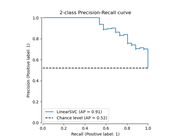
让我们首先在没有分类器预测的情况下绘制精确度-召回率曲线。我们使用 from_estimator,它在绘制曲线之前为我们计算预测结果。
from sklearn.metrics import PrecisionRecallDisplay

display = PrecisionRecallDisplay.from_estimator(
    classifier, X_test, y_test, name="LinearSVC", plot_chance_level=True, despine=True
)
_ = display.ax_.set_title("2-class Precision-Recall curve")

如果我们已经获得了模型的估计概率或分数,那么我们可以使用 from_predictions。
y_score = classifier.decision_function(X_test)

display = PrecisionRecallDisplay.from_predictions(
    y_test, y_score, name="LinearSVC", plot_chance_level=True, despine=True
)
_ = display.ax_.set_title("2-class Precision-Recall curve")
在多标签设置中#
精确度-召回率曲线不支持多标签设置。但是,可以决定如何处理这种情况。我们将在下面展示这样一个示例。
创建多标签数据、拟合和预测#
我们创建一个多标签数据集,以说明多标签设置中的精确度-召回率。
from sklearn.preprocessing import label_binarize

# Use label_binarize to be multi-label like settings
Y = label_binarize(y, classes=[0, 1, 2])
n_classes = Y.shape[1]

# Split into training and test
X_train, X_test, Y_train, Y_test = train_test_split(
    X, Y, test_size=0.5, random_state=random_state
)
我们使用 OneVsRestClassifier 进行多标签预测。
from sklearn.multiclass import OneVsRestClassifier

classifier = OneVsRestClassifier(
    make_pipeline(StandardScaler(), LinearSVC(random_state=random_state))
)
classifier.fit(X_train, Y_train)
y_score = classifier.decision_function(X_test)
多标签设置中的平均精确度得分#
from sklearn.metrics import average_precision_score, precision_recall_curve

# For each class
precision = dict()
recall = dict()
average_precision = dict()
for i in range(n_classes):
    precision[i], recall[i], _ = precision_recall_curve(Y_test[:, i], y_score[:, i])
    average_precision[i] = average_precision_score(Y_test[:, i], y_score[:, i])

# A "micro-average": quantifying score on all classes jointly
precision["micro"], recall["micro"], _ = precision_recall_curve(
    Y_test.ravel(), y_score.ravel()
)
average_precision["micro"] = average_precision_score(Y_test, y_score, average="micro")
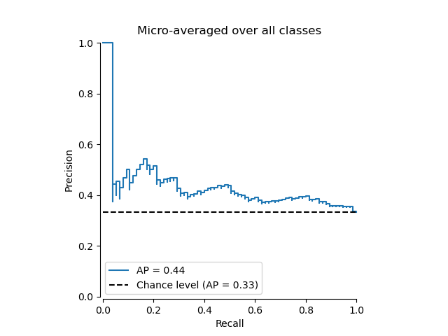
绘制微平均精确度-召回率曲线#
from collections import Counter

display = PrecisionRecallDisplay(
    recall=recall["micro"],
    precision=precision["micro"],
    average_precision=average_precision["micro"],
    prevalence_pos_label=Counter(Y_test.ravel())[1] / Y_test.size,
)
display.plot(plot_chance_level=True, despine=True)
_ = display.ax_.set_title("Micro-averaged over all classes")
绘制每个类别的精确度-召回率曲线和 iso-f1 曲线#
from itertools import cycle

import matplotlib.pyplot as plt

# setup plot details
colors = cycle(["navy", "turquoise", "darkorange", "cornflowerblue", "teal"])

_, ax = plt.subplots(figsize=(7, 8))

f_scores = np.linspace(0.2, 0.8, num=4)
lines, labels = [], []
for f_score in f_scores:
    x = np.linspace(0.01, 1)
    y = f_score * x / (2 * x - f_score)
    (l,) = plt.plot(x[y >= 0], y[y >= 0], color="gray", alpha=0.2)
    plt.annotate("f1={0:0.1f}".format(f_score), xy=(0.9, y[45] + 0.02))

display = PrecisionRecallDisplay(
    recall=recall["micro"],
    precision=precision["micro"],
    average_precision=average_precision["micro"],
)
display.plot(ax=ax, name="Micro-average precision-recall", color="gold")

for i, color in zip(range(n_classes), colors):
    display = PrecisionRecallDisplay(
        recall=recall[i],
        precision=precision[i],
        average_precision=average_precision[i],
    )
    display.plot(
        ax=ax, name=f"Precision-recall for class {i}", color=color, despine=True
    )

# add the legend for the iso-f1 curves
handles, labels = display.ax_.get_legend_handles_labels()
handles.extend([l])
labels.extend(["iso-f1 curves"])
# set the legend and the axes
ax.legend(handles=handles, labels=labels, loc="best")
ax.set_title("Extension of Precision-Recall curve to multi-class")

plt.show()

脚本总运行时间: (0 minutes 2.113 seconds)
相关示例