SparseRandomProjection#
- class sklearn.random_projection.SparseRandomProjection(n_components='auto', *, density='auto', eps=0.1, dense_output=False, compute_inverse_components=False, random_state=None)[source]#
通过稀疏随机投影降低维度。
稀疏随机矩阵是密集随机投影矩阵的替代方案,它保证了相似的嵌入质量,同时内存效率更高,并且允许更快地计算投影数据。
如果我们将
s = 1 / density记作随机矩阵的组件,则这些组件是从以下分布中抽取的-sqrt(s) / sqrt(n_components) with probability 1 / 2s 0 with probability 1 - 1 / s +sqrt(s) / sqrt(n_components) with probability 1 / 2s
在用户指南中了解更多信息。
在版本 0.13 中添加。
- 参数:
- n_componentsint or ‘auto’, default=’auto’
目标投影空间的维度。
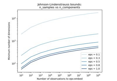
n_components 可以根据数据集中的样本数量和 Johnson-Lindenstrauss 引理给出的边界自动调整。在这种情况下,嵌入的质量由
eps参数控制。需要注意的是,Johnson-Lindenstrauss 引理对所需组件数量的估计可能非常保守,因为它不对数据集的结构做任何假设。
- densityfloat or ‘auto’, default=’auto’
随机投影矩阵中非零组件的比例,范围在 (0, 1] 之间。
如果 density = 'auto',则该值设置为 Ping Li 等人推荐的最小密度:1 / sqrt(n_features)。
如果要重现 Achlioptas, 2001 的结果,请使用 density = 1 / 3.0。
- epsfloat, default=0.1
当 n_components 设置为 'auto' 时,根据 Johnson-Lindenstrauss 引理控制嵌入质量的参数。该值必须严格为正。
值越小,嵌入质量越好,目标投影空间中的维度(n_components)越高。
- dense_outputbool, default=False
如果为 True,即使输入和随机投影矩阵都是稀疏的,也确保随机投影的输出是一个密集 numpy 数组。实际上,如果组件数量很少,则投影数据中的零组件数量将非常少,使用密集表示将更节省 CPU 和内存。
如果为 False,如果输入是稀疏的,则投影数据使用稀疏表示。
- compute_inverse_componentsbool, default=False
通过在 fit 期间计算组件的伪逆来学习逆变换。请注意,伪逆始终是密集数组,即使训练数据是稀疏的也是如此。这意味着可能需要一次在少量样本上调用
inverse_transform以避免耗尽主机上的可用内存。此外,计算伪逆对于大型矩阵的扩展性不好。- random_stateint, RandomState instance or None, default=None
控制用于在 fit 时生成投影矩阵的伪随机数生成器。传递一个 int 以在多次函数调用中获得可重现的输出。请参阅词汇表。
- 属性:
- n_components_int
当 n_components="auto" 时计算出的具体组件数量。
- components_sparse matrix of shape (n_components, n_features)
用于投影的随机矩阵。稀疏矩阵将采用 CSR 格式。
- inverse_components_ndarray of shape (n_features, n_components)
组件的伪逆,仅当
compute_inverse_components为 True 时计算。版本 1.1 中新增。
- density_float in range 0.0 - 1.0
当 density = "auto" 时计算出的具体密度。
- n_features_in_int
在 拟合 期间看到的特征数。
0.24 版本新增。
- feature_names_in_shape 为 (
n_features_in_,) 的 ndarray 在 fit 期间看到的特征名称。仅当
X具有全部为字符串的特征名称时才定义。1.0 版本新增。
另请参阅
GaussianRandomProjection通过高斯随机投影降低维度。
References
[1]Ping Li, T. Hastie and K. W. Church, 2006, “Very Sparse Random Projections”. https://web.stanford.edu/~hastie/Papers/Ping/KDD06_rp.pdf
[2]D. Achlioptas, 2001, “Database-friendly random projections”, https://cgi.di.uoa.gr/~optas/papers/jl.pdf
示例
>>> import numpy as np
>>> from sklearn.random_projection import SparseRandomProjection
>>> rng = np.random.RandomState(42)
>>> X = rng.rand(25, 3000)
>>> transformer = SparseRandomProjection(random_state=rng)
>>> X_new = transformer.fit_transform(X)
>>> X_new.shape
(25, 2759)
>>> # very few components are non-zero
>>> np.mean(transformer.components_ != 0)
np.float64(0.0182)
- fit(X, y=None)[source]#
生成稀疏随机投影矩阵。
- 参数:
- X{ndarray, sparse matrix} of shape (n_samples, n_features)
训练集:仅使用形状来根据上述论文中引用的理论找到最佳随机矩阵维度。
- y被忽略
Not used, present here for API consistency by convention.
- 返回:
- selfobject
BaseRandomProjection 类实例。
- fit_transform(X, y=None, **fit_params)[source]#
拟合数据,然后对其进行转换。
使用可选参数
fit_params将转换器拟合到X和y,并返回X的转换版本。- 参数:
- Xshape 为 (n_samples, n_features) 的 array-like
输入样本。
- y形状为 (n_samples,) 或 (n_samples, n_outputs) 的类数组对象,默认=None
目标值(对于无监督转换,为 None)。
- **fit_paramsdict
额外的拟合参数。仅当估计器在其
fit方法中接受额外的参数时才传递。
- 返回:
- X_newndarray array of shape (n_samples, n_features_new)
转换后的数组。
- get_feature_names_out(input_features=None)[source]#
获取转换的输出特征名称。
The feature names out will prefixed by the lowercased class name. For example, if the transformer outputs 3 features, then the feature names out are:
["class_name0", "class_name1", "class_name2"].- 参数:
- input_featuresarray-like of str or None, default=None
Only used to validate feature names with the names seen in
fit.
- 返回:
- feature_names_outstr 对象的 ndarray
转换后的特征名称。
- get_metadata_routing()[source]#
获取此对象的元数据路由。
请查阅 用户指南,了解路由机制如何工作。
- 返回:
- routingMetadataRequest
封装路由信息的
MetadataRequest。
- get_params(deep=True)[source]#
获取此估计器的参数。
- 参数:
- deepbool, default=True
如果为 True,将返回此估计器以及包含的子对象(如果它们是估计器)的参数。
- 返回:
- paramsdict
参数名称映射到其值。
- inverse_transform(X)[source]#
将数据投影回其原始空间。
返回一个数组 X_original,其变换结果将是 X。请注意,即使 X 是稀疏的,X_original 也是密集的:这可能会占用大量 RAM。
如果
compute_inverse_components为 False,则在每次调用inverse_transform期间都会计算组件的逆,这可能会很耗时。- 参数:
- X{array-like, sparse matrix} of shape (n_samples, n_components)
要逆变换回的数据。
- 返回:
- X_original形状为 (n_samples, n_features) 的 ndarray
重建的数据。
- set_output(*, transform=None)[source]#
设置输出容器。
有关如何使用 API 的示例,请参阅引入 set_output API。
- 参数:
- transform{“default”, “pandas”, “polars”}, default=None
配置
transform和fit_transform的输出。"default": 转换器的默认输出格式"pandas": DataFrame 输出"polars": Polars 输出None: 转换配置保持不变
1.4 版本新增: 添加了
"polars"选项。
- 返回:
- selfestimator instance
估计器实例。