注意
访问结尾 下载完整的示例代码。或通过 JupyterLite 或 Binder 在浏览器中运行此示例
识别手写数字#
此示例演示了如何使用 scikit-learn 来识别手写数字(0-9)的图像。
# Authors: The scikit-learn developers
# SPDX-License-Identifier: BSD-3-Clause

# Standard scientific Python imports
import matplotlib.pyplot as plt

# Import datasets, classifiers and performance metrics
from sklearn import datasets, metrics, svm
from sklearn.model_selection import train_test_split
数字数据集#
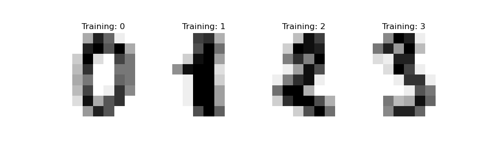
数字数据集包含 8x8 像素的数字图像。数据集的 images 属性存储每个图像的 8x8 灰度值数组。我们将使用这些数组来可视化前 4 幅图像。target 属性存储每个图像代表的数字,这包含在下面 4 个图的标题中。
注意:如果我们使用图像文件(例如“png”文件),我们将使用 matplotlib.pyplot.imread 加载它们。
digits = datasets.load_digits()

_, axes = plt.subplots(nrows=1, ncols=4, figsize=(10, 3))
for ax, image, label in zip(axes, digits.images, digits.target):
    ax.set_axis_off()
    ax.imshow(image, cmap=plt.cm.gray_r, interpolation="nearest")
    ax.set_title("Training: %i" % label)
分类#
要在这个数据上应用分类器,我们需要展平图像,将每个形状为 (8, 8) 的二维灰度值数组转换为形状为 (64,) 的数组。随后,整个数据集的形状将为 (n_samples, n_features),其中 n_samples 是图像数量,n_features 是每幅图像的像素总数。
然后,我们可以将数据分成训练集和测试集,并在训练样本上拟合支持向量机分类器。随后,可以使用拟合后的分类器来预测测试集样本中数字的值。
# flatten the images
n_samples = len(digits.images)
data = digits.images.reshape((n_samples, -1))

# Create a classifier: a support vector classifier
clf = svm.SVC(gamma=0.001)

# Split data into 50% train and 50% test subsets
X_train, X_test, y_train, y_test = train_test_split(
    data, digits.target, test_size=0.5, shuffle=False
)

# Learn the digits on the train subset
clf.fit(X_train, y_train)

# Predict the value of the digit on the test subset
predicted = clf.predict(X_test)
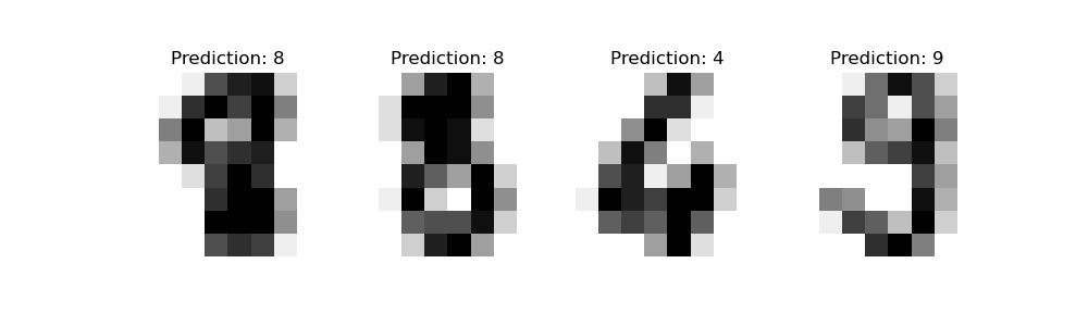
下面,我们可视化前 4 个测试样本,并在标题中显示它们的预测数字值。
_, axes = plt.subplots(nrows=1, ncols=4, figsize=(10, 3))
for ax, image, prediction in zip(axes, X_test, predicted):
    ax.set_axis_off()
    image = image.reshape(8, 8)
    ax.imshow(image, cmap=plt.cm.gray_r, interpolation="nearest")
    ax.set_title(f"Prediction: {prediction}")
classification_report 构建一个文本报告,显示主要的分类指标。
print(
    f"Classification report for classifier {clf}:\n"
    f"{metrics.classification_report(y_test, predicted)}\n"
)
Classification report for classifier SVC(gamma=0.001):
              precision    recall  f1-score   support

           0       1.00      0.99      0.99        88
           1       0.99      0.97      0.98        91
           2       0.99      0.99      0.99        86
           3       0.98      0.87      0.92        91
           4       0.99      0.96      0.97        92
           5       0.95      0.97      0.96        91
           6       0.99      0.99      0.99        91
           7       0.96      0.99      0.97        89
           8       0.94      1.00      0.97        88
           9       0.93      0.98      0.95        92

    accuracy                           0.97       899
   macro avg       0.97      0.97      0.97       899
weighted avg       0.97      0.97      0.97       899
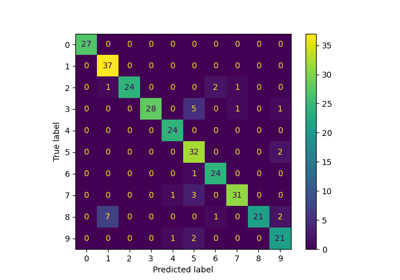
我们还可以绘制真实数字值和预测数字值的 混淆矩阵。
disp = metrics.ConfusionMatrixDisplay.from_predictions(y_test, predicted)
disp.figure_.suptitle("Confusion Matrix")
print(f"Confusion matrix:\n{disp.confusion_matrix}")

plt.show()
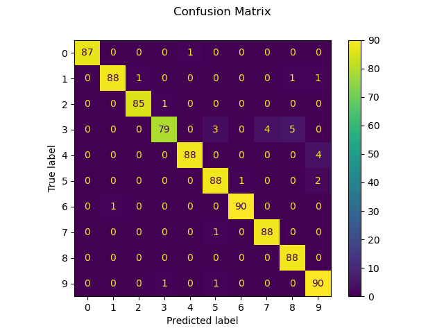
Confusion matrix:
[[87  0  0  0  1  0  0  0  0  0]
 [ 0 88  1  0  0  0  0  0  1  1]
 [ 0  0 85  1  0  0  0  0  0  0]
 [ 0  0  0 79  0  3  0  4  5  0]
 [ 0  0  0  0 88  0  0  0  0  4]
 [ 0  0  0  0  0 88  1  0  0  2]
 [ 0  1  0  0  0  0 90  0  0  0]
 [ 0  0  0  0  0  1  0 88  0  0]
 [ 0  0  0  0  0  0  0  0 88  0]
 [ 0  0  0  1  0  1  0  0  0 90]]
如果评估分类器的结果以 混淆矩阵 的形式存储,而不是 y_true 和 y_pred 的形式,仍然可以构建 classification_report,如下所示
# The ground truth and predicted lists
y_true = []
y_pred = []
cm = disp.confusion_matrix

# For each cell in the confusion matrix, add the corresponding ground truths
# and predictions to the lists
for gt in range(len(cm)):
    for pred in range(len(cm)):
        y_true += [gt] * cm[gt][pred]
        y_pred += [pred] * cm[gt][pred]

print(
    "Classification report rebuilt from confusion matrix:\n"
    f"{metrics.classification_report(y_true, y_pred)}\n"
)
Classification report rebuilt from confusion matrix:
              precision    recall  f1-score   support

           0       1.00      0.99      0.99        88
           1       0.99      0.97      0.98        91
           2       0.99      0.99      0.99        86
           3       0.98      0.87      0.92        91
           4       0.99      0.96      0.97        92
           5       0.95      0.97      0.96        91
           6       0.99      0.99      0.99        91
           7       0.96      0.99      0.97        89
           8       0.94      1.00      0.97        88
           9       0.93      0.98      0.95        92

    accuracy                           0.97       899
   macro avg       0.97      0.97      0.97       899
weighted avg       0.97      0.97      0.97       899
脚本总运行时间:(0 分钟 0.435 秒)
相关示例