使用概率 PCA 和因子分析 (FA) 进行模型选择#

概率PCA和因子分析是概率模型。因此，新数据的似然性可以用于模型选择和协方差估计。在这里，我们将PCA和FA与交叉验证进行比较，数据为低秩数据，并加入同方差噪声（每个特征的噪声方差相同）或异方差噪声（每个特征的噪声方差不同）。第二步，我们将模型似然性与收缩协方差估计量获得的似然性进行比较。

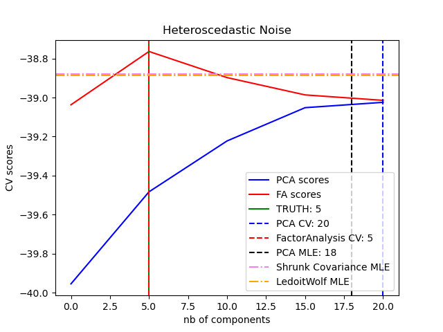
可以观察到，在同方差噪声下，FA和PCA都能成功地恢复低秩子空间的大小。在这种情况下，PCA的似然性高于FA。然而，当存在异方差噪声时，PCA会失败并高估秩。在适当的情况下（组件数量的选择），对于低秩模型，保留数据的可能性高于收缩模型。

还将与Thomas P. Minka的《自动选择PCA的维度》 (Automatic Choice of Dimensionality for PCA. NIPS 2000: 598-604) 中的自动估计方法进行比较。

# Authors: The scikit-learn developers
# SPDX-License-Identifier: BSD-3-Clause

创建数据#

import numpy as np
from scipy import linalg

n_samples, n_features, rank = 500, 25, 5
sigma = 1.0
rng = np.random.RandomState(42)
U, _, _ = linalg.svd(rng.randn(n_features, n_features))
X = np.dot(rng.randn(n_samples, rank), U[:, :rank].T)

# Adding homoscedastic noise
X_homo = X + sigma * rng.randn(n_samples, n_features)

# Adding heteroscedastic noise
sigmas = sigma * rng.rand(n_features) + sigma / 2.0
X_hetero = X + rng.randn(n_samples, n_features) * sigmas

拟合模型#

import matplotlib.pyplot as plt

from sklearn.covariance import LedoitWolf, ShrunkCovariance
from sklearn.decomposition import PCA, FactorAnalysis
from sklearn.model_selection import GridSearchCV, cross_val_score

n_components = np.arange(0, n_features, 5)  # options for n_components


def compute_scores(X):
    pca = PCA(svd_solver="full")
    fa = FactorAnalysis()

    pca_scores, fa_scores = [], []
    for n in n_components:
        pca.n_components = n
        fa.n_components = n
        pca_scores.append(np.mean(cross_val_score(pca, X)))
        fa_scores.append(np.mean(cross_val_score(fa, X)))

    return pca_scores, fa_scores


def shrunk_cov_score(X):
    shrinkages = np.logspace(-2, 0, 30)
    cv = GridSearchCV(ShrunkCovariance(), {"shrinkage": shrinkages})
    return np.mean(cross_val_score(cv.fit(X).best_estimator_, X))


def lw_score(X):
    return np.mean(cross_val_score(LedoitWolf(), X))


for X, title in [(X_homo, "Homoscedastic Noise"), (X_hetero, "Heteroscedastic Noise")]:
    pca_scores, fa_scores = compute_scores(X)
    n_components_pca = n_components[np.argmax(pca_scores)]
    n_components_fa = n_components[np.argmax(fa_scores)]

    pca = PCA(svd_solver="full", n_components="mle")
    pca.fit(X)
    n_components_pca_mle = pca.n_components_

    print("best n_components by PCA CV = %d" % n_components_pca)
    print("best n_components by FactorAnalysis CV = %d" % n_components_fa)
    print("best n_components by PCA MLE = %d" % n_components_pca_mle)

    plt.figure()
    plt.plot(n_components, pca_scores, "b", label="PCA scores")
    plt.plot(n_components, fa_scores, "r", label="FA scores")
    plt.axvline(rank, color="g", label="TRUTH: %d" % rank, linestyle="-")
    plt.axvline(
        n_components_pca,
        color="b",
        label="PCA CV: %d" % n_components_pca,
        linestyle="--",
    )
    plt.axvline(
        n_components_fa,
        color="r",
        label="FactorAnalysis CV: %d" % n_components_fa,
        linestyle="--",
    )
    plt.axvline(
        n_components_pca_mle,
        color="k",
        label="PCA MLE: %d" % n_components_pca_mle,
        linestyle="--",
    )

    # compare with other covariance estimators
    plt.axhline(
        shrunk_cov_score(X),
        color="violet",
        label="Shrunk Covariance MLE",
        linestyle="-.",
    )
    plt.axhline(
        lw_score(X),
        color="orange",
        label="LedoitWolf MLE" % n_components_pca_mle,
        linestyle="-.",
    )

    plt.xlabel("nb of components")
    plt.ylabel("CV scores")
    plt.legend(loc="lower right")
    plt.title(title)

plt.show()

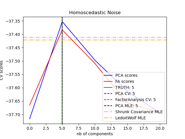
best n_components by PCA CV = 5
best n_components by FactorAnalysis CV = 5
best n_components by PCA MLE = 5
best n_components by PCA CV = 20
best n_components by FactorAnalysis CV = 5
best n_components by PCA MLE = 18

脚本总运行时间：（0分钟3.135秒）