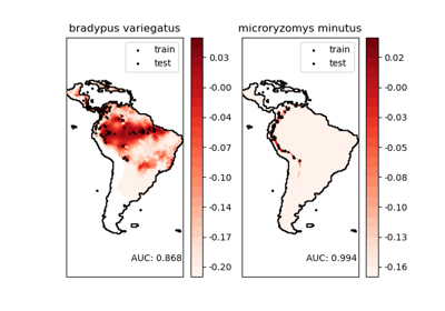
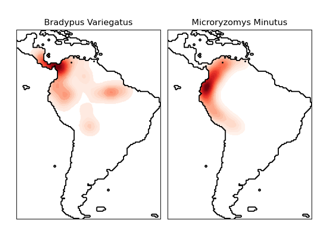
物种分布的核密度估计

此示例演示了基于邻居的查询（特别是核密度估计）在地理空间数据上的应用，使用基于 Haversine 距离度量的球树——即经纬度点上的距离。数据集由 Phillips 等人提供。(2006)。如果可用，该示例使用 basemap 绘制南美洲的海岸线和国家边界。

此示例不执行任何数据学习（参见 物种分布建模，了解基于此数据集中属性的分类示例）。它只显示地理空间坐标中观察到的数据点的核密度估计。

这两种物种是

• “Bradypus variegatus”，即棕喉树懒。

• “Microryzomys minutus”，也称为森林小型稻鼠，一种生活在秘鲁、哥伦比亚、厄瓜多尔、秘鲁和委内瑞拉的啮齿动物。

参考文献

• “物种地理分布的最大熵建模” S. J. Phillips, R. P. Anderson, R. E. Schapire - 生态建模，190:231-259, 2006。

- computing KDE in spherical coordinates
- plot coastlines from coverage
- computing KDE in spherical coordinates
- plot coastlines from coverage

# Authors: The scikit-learn developers
# SPDX-License-Identifier: BSD-3-Clause

import matplotlib.pyplot as plt
import numpy as np

from sklearn.datasets import fetch_species_distributions
from sklearn.neighbors import KernelDensity

# if basemap is available, we'll use it.
# otherwise, we'll improvise later...
try:
    from mpl_toolkits.basemap import Basemap

    basemap = True
except ImportError:
    basemap = False


def construct_grids(batch):
    """Construct the map grid from the batch object

    Parameters
    ----------
    batch : Batch object
        The object returned by :func:`fetch_species_distributions`

    Returns
    -------
    (xgrid, ygrid) : 1-D arrays
        The grid corresponding to the values in batch.coverages
    """
    # x,y coordinates for corner cells
    xmin = batch.x_left_lower_corner + batch.grid_size
    xmax = xmin + (batch.Nx * batch.grid_size)
    ymin = batch.y_left_lower_corner + batch.grid_size
    ymax = ymin + (batch.Ny * batch.grid_size)

    # x coordinates of the grid cells
    xgrid = np.arange(xmin, xmax, batch.grid_size)
    # y coordinates of the grid cells
    ygrid = np.arange(ymin, ymax, batch.grid_size)

    return (xgrid, ygrid)


# Get matrices/arrays of species IDs and locations
data = fetch_species_distributions()
species_names = ["Bradypus Variegatus", "Microryzomys Minutus"]

Xtrain = np.vstack([data["train"]["dd lat"], data["train"]["dd long"]]).T
ytrain = np.array(
    [d.decode("ascii").startswith("micro") for d in data["train"]["species"]],
    dtype="int",
)
Xtrain *= np.pi / 180.0  # Convert lat/long to radians

# Set up the data grid for the contour plot
xgrid, ygrid = construct_grids(data)
X, Y = np.meshgrid(xgrid[::5], ygrid[::5][::-1])
land_reference = data.coverages[6][::5, ::5]
land_mask = (land_reference > -9999).ravel()

xy = np.vstack([Y.ravel(), X.ravel()]).T
xy = xy[land_mask]
xy *= np.pi / 180.0

# Plot map of South America with distributions of each species
fig = plt.figure()
fig.subplots_adjust(left=0.05, right=0.95, wspace=0.05)

for i in range(2):
    plt.subplot(1, 2, i + 1)

    # construct a kernel density estimate of the distribution
    print(" - computing KDE in spherical coordinates")
    kde = KernelDensity(
        bandwidth=0.04, metric="haversine", kernel="gaussian", algorithm="ball_tree"
    )
    kde.fit(Xtrain[ytrain == i])

    # evaluate only on the land: -9999 indicates ocean
    Z = np.full(land_mask.shape[0], -9999, dtype="int")
    Z[land_mask] = np.exp(kde.score_samples(xy))
    Z = Z.reshape(X.shape)

    # plot contours of the density
    levels = np.linspace(0, Z.max(), 25)
    plt.contourf(X, Y, Z, levels=levels, cmap=plt.cm.Reds)

    if basemap:
        print(" - plot coastlines using basemap")
        m = Basemap(
            projection="cyl",
            llcrnrlat=Y.min(),
            urcrnrlat=Y.max(),
            llcrnrlon=X.min(),
            urcrnrlon=X.max(),
            resolution="c",
        )
        m.drawcoastlines()
        m.drawcountries()
    else:
        print(" - plot coastlines from coverage")
        plt.contour(
            X, Y, land_reference, levels=[-9998], colors="k", linestyles="solid"
        )
        plt.xticks([])
        plt.yticks([])

    plt.title(species_names[i])

plt.show()

相关示例

物种分布模型

物种分布模型

核密度估计

核密度估计

SGD：加权样本

SGD：加权样本

简单的 1D 核密度估计

简单的 1D 核密度估计