标签传播数字：演示性能#

此示例通过训练标签传播模型来对带有极少量标签的手写数字进行分类，从而演示半监督学习的强大功能。

手写数字数据集共有 1797 个点。模型将使用所有点进行训练，但只有 30 个点将被标记。结果将以混淆矩阵和每个类别的系列指标的形式呈现，效果非常好。

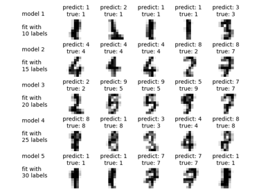
最后，将显示前 10 个最不确定的预测。

# Authors: The scikit-learn developers
# SPDX-License-Identifier: BSD-3-Clause

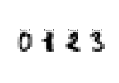
数据生成#

我们使用 digits 数据集。我们只使用随机选择的样本子集。

import numpy as np

from sklearn import datasets

digits = datasets.load_digits()
rng = np.random.RandomState(2)
indices = np.arange(len(digits.data))
rng.shuffle(indices)

我们选择了 340 个样本，其中只有 40 个样本与已知标签相关联。因此，我们存储了另外 300 个样本的索引，我们不应该知道它们的标签。

X = digits.data[indices[:340]]
y = digits.target[indices[:340]]
images = digits.images[indices[:340]]

n_total_samples = len(y)
n_labeled_points = 40

indices = np.arange(n_total_samples)

unlabeled_set = indices[n_labeled_points:]

随机打乱所有内容

y_train = np.copy(y)
y_train[unlabeled_set] = -1

半监督学习#

我们拟合一个LabelSpreading 并用它来预测未知标签。

from sklearn.metrics import classification_report
from sklearn.semi_supervised import LabelSpreading

lp_model = LabelSpreading(gamma=0.25, max_iter=20)
lp_model.fit(X, y_train)
predicted_labels = lp_model.transduction_[unlabeled_set]
true_labels = y[unlabeled_set]

print(
    "Label Spreading model: %d labeled & %d unlabeled points (%d total)"
    % (n_labeled_points, n_total_samples - n_labeled_points, n_total_samples)
)

Label Spreading model: 40 labeled & 300 unlabeled points (340 total)

分类报告

print(classification_report(true_labels, predicted_labels))

              precision    recall  f1-score   support

           0       1.00      1.00      1.00        27
           1       0.82      1.00      0.90        37
           2       1.00      0.86      0.92        28
           3       1.00      0.80      0.89        35
           4       0.92      1.00      0.96        24
           5       0.74      0.94      0.83        34
           6       0.89      0.96      0.92        25
           7       0.94      0.89      0.91        35
           8       1.00      0.68      0.81        31
           9       0.81      0.88      0.84        24

    accuracy                           0.90       300
   macro avg       0.91      0.90      0.90       300
weighted avg       0.91      0.90      0.90       300

混淆矩阵

from sklearn.metrics import ConfusionMatrixDisplay

ConfusionMatrixDisplay.from_predictions(
    true_labels, predicted_labels, labels=lp_model.classes_
)

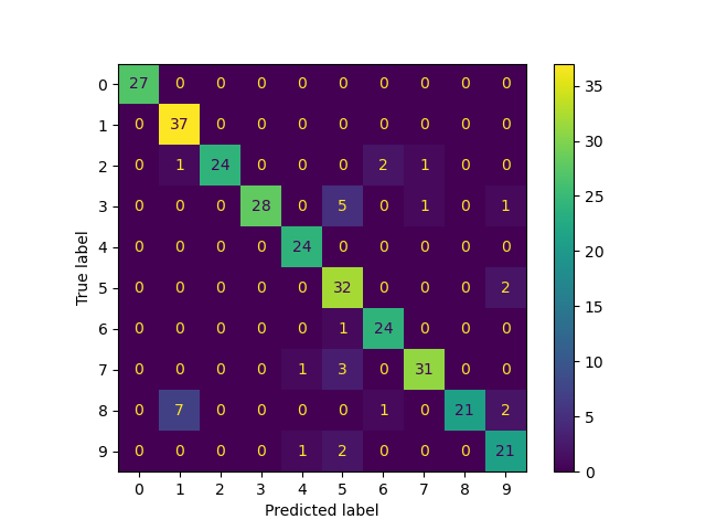
<sklearn.metrics._plot.confusion_matrix.ConfusionMatrixDisplay object at 0x74b4a9371940>

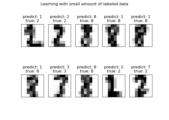
绘制最不确定的预测#

在这里，我们将挑选并显示 10 个最不确定的预测。

from scipy import stats

pred_entropies = stats.distributions.entropy(lp_model.label_distributions_.T)

挑选前 10 个最不确定的标签

uncertainty_index = np.argsort(pred_entropies)[-10:]

绘图

import matplotlib.pyplot as plt

f = plt.figure(figsize=(7, 5))
for index, image_index in enumerate(uncertainty_index):
    image = images[image_index]

    sub = f.add_subplot(2, 5, index + 1)
    sub.imshow(image, cmap=plt.cm.gray_r)
    plt.xticks([])
    plt.yticks([])
    sub.set_title(
        "predict: %i\ntrue: %i" % (lp_model.transduction_[image_index], y[image_index])
    )

f.suptitle("Learning with small amount of labeled data")
plt.show()

Learning with small amount of labeled data, predict: 1 true: 2, predict: 2 true: 2, predict: 8 true: 8, predict: 1 true: 8, predict: 1 true: 8, predict: 1 true: 8, predict: 3 true: 3, predict: 8 true: 8, predict: 2 true: 2, predict: 7 true: 2

脚本总运行时间：（0 分钟 0.401 秒）