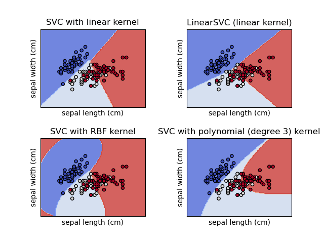
在鸢尾花数据集上绘制不同的 SVM 分类器#

比较鸢尾花数据集的二维投影上不同线性 SVM 分类器的效果。我们只考虑该数据集的前两个特征。

萼片长度
萼片宽度

此示例演示如何绘制具有不同内核的四个 SVM 分类器的决策面。

线性模型 LinearSVC() 和 SVC(kernel='linear') 会产生略微不同的决策边界。这可能是以下差异的结果：

LinearSVC 最小化平方合页损失，而 SVC 最小化正则合页损失。
LinearSVC 使用一对多 (也称为一对其余) 多类归约，而 SVC 使用一对一多类归约。

两个线性模型都具有线性决策边界（相交超平面），而非线性核模型（多项式或高斯 RBF）具有更灵活的非线性决策边界，其形状取决于核的类型及其参数。

注意

虽然绘制玩具二维数据集的分类器的决策函数可以帮助直观地理解它们各自的表达能力，但请注意，这些直觉并不总是能够推广到更现实的高维问题。

SVC with linear kernel, LinearSVC (linear kernel), SVC with RBF kernel, SVC with polynomial (degree 3) kernel

# Authors: The scikit-learn developers
# SPDX-License-Identifier: BSD-3-Clause

import matplotlib.pyplot as plt

from sklearn import datasets, svm
from sklearn.inspection import DecisionBoundaryDisplay

# import some data to play with
iris = datasets.load_iris()
# Take the first two features. We could avoid this by using a two-dim dataset
X = iris.data[:, :2]
y = iris.target

# we create an instance of SVM and fit out data. We do not scale our
# data since we want to plot the support vectors
C = 1.0  # SVM regularization parameter
models = (
    svm.SVC(kernel="linear", C=C),
    svm.LinearSVC(C=C, max_iter=10000),
    svm.SVC(kernel="rbf", gamma=0.7, C=C),
    svm.SVC(kernel="poly", degree=3, gamma="auto", C=C),
)
models = (clf.fit(X, y) for clf in models)

# title for the plots
titles = (
    "SVC with linear kernel",
    "LinearSVC (linear kernel)",
    "SVC with RBF kernel",
    "SVC with polynomial (degree 3) kernel",
)

# Set-up 2x2 grid for plotting.
fig, sub = plt.subplots(2, 2)
plt.subplots_adjust(wspace=0.4, hspace=0.4)

X0, X1 = X[:, 0], X[:, 1]

for clf, title, ax in zip(models, titles, sub.flatten()):
    disp = DecisionBoundaryDisplay.from_estimator(
        clf,
        X,
        response_method="predict",
        cmap=plt.cm.coolwarm,
        alpha=0.8,
        ax=ax,
        xlabel=iris.feature_names[0],
        ylabel=iris.feature_names[1],
    )
    ax.scatter(X0, X1, c=y, cmap=plt.cm.coolwarm, s=20, edgecolors="k")
    ax.set_xticks(())
    ax.set_yticks(())
    ax.set_title(title)

plt.show()

脚本的总运行时间：（0 分钟 0.207 秒）