逻辑回归中的 L1 正则化和稀疏性#

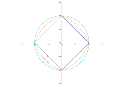
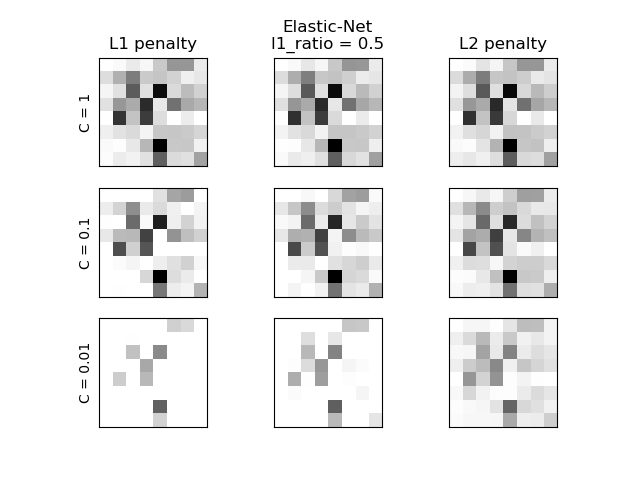
当使用L1、L2和Elastic-Net惩罚项时，不同C值下解的稀疏度（零系数的百分比）比较。我们可以看到，较大的C值给予模型更大的自由度。相反，较小的C值对模型的约束更大。在L1惩罚项的情况下，这会导致更稀疏的解。正如预期的那样，Elastic-Net惩罚项的稀疏度介于L1和L2之间。

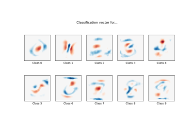
我们将8x8的数字图像分为两类：0-4和5-9。可视化显示了不同C值下模型的系数。

L1 penalty, Elastic-Net l1_ratio = 0.5, L2 penalty

C=1.00
Sparsity with L1 penalty:                4.69%
Sparsity with Elastic-Net penalty:       4.69%
Sparsity with L2 penalty:                4.69%
Score with L1 penalty:                   0.90
Score with Elastic-Net penalty:          0.90
Score with L2 penalty:                   0.90
C=0.10
Sparsity with L1 penalty:                29.69%
Sparsity with Elastic-Net penalty:       14.06%
Sparsity with L2 penalty:                4.69%
Score with L1 penalty:                   0.90
Score with Elastic-Net penalty:          0.90
Score with L2 penalty:                   0.90
C=0.01
Sparsity with L1 penalty:                84.38%
Sparsity with Elastic-Net penalty:       68.75%
Sparsity with L2 penalty:                4.69%
Score with L1 penalty:                   0.86
Score with Elastic-Net penalty:          0.88
Score with L2 penalty:                   0.89

# Authors: The scikit-learn developers
# SPDX-License-Identifier: BSD-3-Clause

import matplotlib.pyplot as plt
import numpy as np

from sklearn import datasets
from sklearn.linear_model import LogisticRegression
from sklearn.preprocessing import StandardScaler

X, y = datasets.load_digits(return_X_y=True)

X = StandardScaler().fit_transform(X)

# classify small against large digits
y = (y > 4).astype(int)

l1_ratio = 0.5  # L1 weight in the Elastic-Net regularization

fig, axes = plt.subplots(3, 3)

# Set regularization parameter
for i, (C, axes_row) in enumerate(zip((1, 0.1, 0.01), axes)):
    # Increase tolerance for short training time
    clf_l1_LR = LogisticRegression(C=C, penalty="l1", tol=0.01, solver="saga")
    clf_l2_LR = LogisticRegression(C=C, penalty="l2", tol=0.01, solver="saga")
    clf_en_LR = LogisticRegression(
        C=C, penalty="elasticnet", solver="saga", l1_ratio=l1_ratio, tol=0.01
    )
    clf_l1_LR.fit(X, y)
    clf_l2_LR.fit(X, y)
    clf_en_LR.fit(X, y)

    coef_l1_LR = clf_l1_LR.coef_.ravel()
    coef_l2_LR = clf_l2_LR.coef_.ravel()
    coef_en_LR = clf_en_LR.coef_.ravel()

    # coef_l1_LR contains zeros due to the
    # L1 sparsity inducing norm

    sparsity_l1_LR = np.mean(coef_l1_LR == 0) * 100
    sparsity_l2_LR = np.mean(coef_l2_LR == 0) * 100
    sparsity_en_LR = np.mean(coef_en_LR == 0) * 100

    print(f"C={C:.2f}")
    print(f"{'Sparsity with L1 penalty:':<40} {sparsity_l1_LR:.2f}%")
    print(f"{'Sparsity with Elastic-Net penalty:':<40} {sparsity_en_LR:.2f}%")
    print(f"{'Sparsity with L2 penalty:':<40} {sparsity_l2_LR:.2f}%")
    print(f"{'Score with L1 penalty:':<40} {clf_l1_LR.score(X, y):.2f}")
    print(f"{'Score with Elastic-Net penalty:':<40} {clf_en_LR.score(X, y):.2f}")
    print(f"{'Score with L2 penalty:':<40} {clf_l2_LR.score(X, y):.2f}")

    if i == 0:
        axes_row[0].set_title("L1 penalty")
        axes_row[1].set_title("Elastic-Net\nl1_ratio = %s" % l1_ratio)
        axes_row[2].set_title("L2 penalty")

    for ax, coefs in zip(axes_row, [coef_l1_LR, coef_en_LR, coef_l2_LR]):
        ax.imshow(
            np.abs(coefs.reshape(8, 8)),
            interpolation="nearest",
            cmap="binary",
            vmax=1,
            vmin=0,
        )
        ax.set_xticks(())
        ax.set_yticks(())

    axes_row[0].set_ylabel(f"C = {C}")

plt.show()

脚本总运行时间：（0分0.528秒）