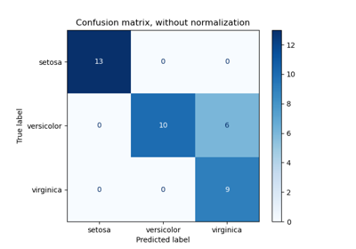
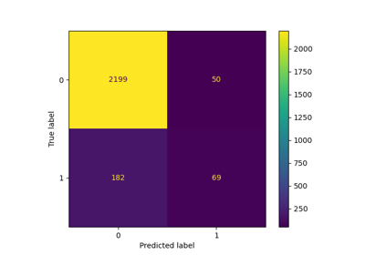
confusion_matrix#
- sklearn.metrics.confusion_matrix(y_true, y_pred, *, labels=None, sample_weight=None, normalize=None)[source]#
计算混淆矩阵以评估分类的准确性。
根据定义,混淆矩阵 \(C\) 满足 \(C_{i, j}\) 等于已知属于组 \(i\) 但预测属于组 \(j\) 的观测值数量。
因此在二分类中,真阴性的数量是 \(C_{0,0}\),假阴性的数量是 \(C_{1,0}\),真阳性的数量是 \(C_{1,1}\),假阳性的数量是 \(C_{0,1}\)。
在用户指南中阅读更多内容。
- 参数:
- y_true形状为 (n_samples,) 的 array-like
真实(正确)的目标值。
- y_pred形状为 (n_samples,) 的类数组
分类器返回的估计目标。
- labels形状为 (n_classes,) 的类数组对象, 默认为 None
用于索引矩阵的标签列表。可用于重新排序或选择标签子集。如果给定
None,则使用出现在y_true或y_pred中至少一次的标签,并按排序顺序排列。- sample_weightshape 为 (n_samples,) 的 array-like, default=None
样本权重。
版本 0.18 新增。
- normalize{‘true’, ‘pred’, ‘all’}, default=None
根据真实条件(行)、预测条件(列)或所有总体对混淆矩阵进行归一化。如果为 None,则混淆矩阵不会被归一化。
- 返回:
- Cndarray of shape (n_classes, n_classes)
混淆矩阵,其第 i 行第 j 列的条目表示真实标签为第 i 类且预测标签为第 j 类的样本数量。
另请参阅
ConfusionMatrixDisplay.from_estimator给定估计器、数据和标签,绘制混淆矩阵。
ConfusionMatrixDisplay.from_predictions给定真实标签和预测标签,绘制混淆矩阵。
ConfusionMatrixDisplay混淆矩阵可视化。
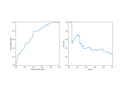
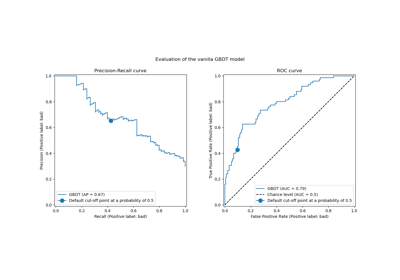
confusion_matrix_at_thresholds对于二分类,计算每个阈值的真阴性、假阳性、假阴性和真阳性计数。
References
[1]混淆矩阵的维基百科条目(维基百科和其他参考资料可能使用不同的轴约定)。
示例
>>> from sklearn.metrics import confusion_matrix
>>> y_true = [2, 0, 2, 2, 0, 1]
>>> y_pred = [0, 0, 2, 2, 0, 2]
>>> confusion_matrix(y_true, y_pred)
array([[2, 0, 0],
       [0, 0, 1],
       [1, 0, 2]])
>>> y_true = ["cat", "ant", "cat", "cat", "ant", "bird"]
>>> y_pred = ["ant", "ant", "cat", "cat", "ant", "cat"]
>>> confusion_matrix(y_true, y_pred, labels=["ant", "bird", "cat"])
array([[2, 0, 0],
       [0, 0, 1],
       [1, 0, 2]])
在二分类情况下,我们可以提取真阳性等如下所示
>>> tn, fp, fn, tp = confusion_matrix([0, 1, 0, 1], [1, 1, 1, 0]).ravel().tolist()
>>> (tn, fp, fn, tp)
(0, 2, 1, 1)