注意
跳到末尾下载完整的示例代码,或通过 JupyterLite 或 Binder 在浏览器中运行此示例。
成本敏感学习的决策阈值后调整#
分类器训练完成后,predict 方法的输出是与 decision_function 或 predict_proba 输出的阈值处理对应的类别标签预测。对于二元分类器,默认阈值定义为后验概率估计值 0.5 或决策分数 0.0。
然而,这种默认策略对于手头的任务很可能不是最优的。在这里,我们使用 “Statlog” 德国信用数据集 [1] 来演示一个用例。在这个数据集中,任务是预测一个人拥有“好”信用还是“坏”信用。此外,还提供了一个成本矩阵,指定了错误分类的成本。具体来说,将“坏”信用错误分类为“好”的成本平均是将来“好”信用错误分类为“坏”的五倍。
我们使用 TunedThresholdClassifierCV 来选择决策函数的截止点,以最小化所提供的业务成本。
在示例的第二部分,我们通过考虑信用卡交易中的欺诈检测问题进一步扩展了此方法:在这种情况下,业务指标取决于每笔交易的金额。
References
# Authors: The scikit-learn developers
# SPDX-License-Identifier: BSD-3-Clause
具有固定收益和成本的成本敏感学习#
在本第一节中,我们将在混淆矩阵的每个条目关联的收益和成本为常数的情况下,演示 TunedThresholdClassifierCV 在成本敏感学习中的使用。我们使用 [2] 中提出的问题,使用 “Statlog” 德国信用数据集 [1]。
“Statlog” 德国信用数据集#
我们从 OpenML 获取德国信用数据集。
import sklearn
from sklearn.datasets import fetch_openml

sklearn.set_config(transform_output="pandas")

german_credit = fetch_openml(data_id=31, as_frame=True, parser="pandas")
X, y = german_credit.data, german_credit.target
我们检查 X 中可用的特征类型。
X.info()
<class 'pandas.core.frame.DataFrame'>
RangeIndex: 1000 entries, 0 to 999
Data columns (total 20 columns):
 #   Column                  Non-Null Count  Dtype
---  ------                  --------------  -----
 0   checking_status         1000 non-null   category
 1   duration                1000 non-null   int64
 2   credit_history          1000 non-null   category
 3   purpose                 1000 non-null   category
 4   credit_amount           1000 non-null   int64
 5   savings_status          1000 non-null   category
 6   employment              1000 non-null   category
 7   installment_commitment  1000 non-null   int64
 8   personal_status         1000 non-null   category
 9   other_parties           1000 non-null   category
 10  residence_since         1000 non-null   int64
 11  property_magnitude      1000 non-null   category
 12  age                     1000 non-null   int64
 13  other_payment_plans     1000 non-null   category
 14  housing                 1000 non-null   category
 15  existing_credits        1000 non-null   int64
 16  job                     1000 non-null   category
 17  num_dependents          1000 non-null   int64
 18  own_telephone           1000 non-null   category
 19  foreign_worker          1000 non-null   category
dtypes: category(13), int64(7)
memory usage: 69.9 KB
许多特征是分类的,通常是字符串编码的。在开发预测模型时,我们需要对这些类别进行编码。让我们检查一下目标。
y.value_counts()
class
good    700
bad     300
Name: count, dtype: int64
另一个观察是数据集不平衡。在评估预测模型时,我们需要小心,并使用一系列适合这种情况的指标。
此外,我们观察到目标是字符串编码的。某些指标(例如,精确率和召回率)需要提供感兴趣的标签,也称为“正标签”。在这里,我们将目标定义为预测样本是否为“不良”信用。
pos_label, neg_label = "bad", "good"
为了进行我们的分析,我们使用单一分层拆分来拆分数据集。
from sklearn.model_selection import train_test_split

X_train, X_test, y_train, y_test = train_test_split(X, y, stratify=y, random_state=0)
我们已准备好设计我们的预测模型和相关的评估策略。
评估指标#
在本节中,我们定义了一组稍后将使用的指标。为了查看调整截止点的影响,我们使用接收者操作特征 (ROC) 曲线和精确率-召回率曲线评估预测模型。这些图上报告的值因此是真阳性率 (TPR),也称为召回率或敏感度,以及假阳性率 (FPR),也称为特异度,用于 ROC 曲线,以及精确率和召回率用于精确率-召回率曲线。
在这四个指标中,scikit-learn 没有提供 FPR 的评分器。因此,我们需要定义一个小的自定义函数来计算它。
from sklearn.metrics import confusion_matrix


def fpr_score(y, y_pred, neg_label, pos_label):
    cm = confusion_matrix(y, y_pred, labels=[neg_label, pos_label])
    tn, fp, _, _ = cm.ravel()
    tnr = tn / (tn + fp)
    return 1 - tnr
如前所述,“正标签”未定义为值“1”,并且用此非标准值调用某些指标会引发错误。我们需要向指标提供“正标签”的指示。
因此,我们需要使用 make_scorer 定义一个 scikit-learn 评分器,其中传递信息。我们将所有自定义评分器存储在一个字典中。要使用它们,我们需要传递拟合的模型、数据和我们想要评估预测模型的目标。
from sklearn.metrics import make_scorer, precision_score, recall_score

tpr_score = recall_score  # TPR and recall are the same metric
scoring = {
    "precision": make_scorer(precision_score, pos_label=pos_label),
    "recall": make_scorer(recall_score, pos_label=pos_label),
    "fpr": make_scorer(fpr_score, neg_label=neg_label, pos_label=pos_label),
    "tpr": make_scorer(tpr_score, pos_label=pos_label),
}
此外,原始研究 [1] 定义了一个自定义业务指标。我们称“业务指标”为旨在量化预测(正确或错误)如何影响在特定应用上下文中部署给定机器学习模型的业务价值的任何指标函数。对于我们的信用预测任务,作者提供了一个自定义成本矩阵,该矩阵编码将“坏”信用分类为“好”的成本平均是相反情况的 5 倍:对于金融机构来说,不向潜在客户授予信用(从而错失了一个本来会偿还信用并支付利息的好客户)的成本要低于向一个会违约的客户授予信用。
我们定义了一个 Python 函数,它对混淆矩阵进行加权并返回总成本。混淆矩阵的行包含观察到的类别的计数,而列包含预测的类别的计数。回想一下,这里我们将“坏”视为正类别(第二行和第二列)。Scikit-learn 模型选择工具期望我们遵循“更高”意味着“更好”的约定,因此以下增益矩阵将负增益(成本)分配给两种预测错误
每个假阳性(将“好”信用标记为“坏”)的收益为
-1,每个假阴性(将“坏”信用标记为“好”)的收益为
-5,真阳性和真阴性的收益为
0。
请注意,从理论上讲,鉴于我们的模型经过校准且数据集具有代表性且足够大,我们无需调整阈值,而是可以安全地将其设置为成本比的 1/5,如 Elkan 论文 [2] 中的公式 (2) 所述。
import numpy as np


def credit_gain_score(y, y_pred, neg_label, pos_label):
    cm = confusion_matrix(y, y_pred, labels=[neg_label, pos_label])

    gain_matrix = np.array(
        [
            [0, -1],  # -1 gain for false positives
            [-5, 0],  # -5 gain for false negatives
        ]
    )
    return np.sum(cm * gain_matrix)


scoring["credit_gain"] = make_scorer(
    credit_gain_score, neg_label=neg_label, pos_label=pos_label
)
普通预测模型#
我们使用 HistGradientBoostingClassifier 作为预测模型,它原生处理分类特征和缺失值。
from sklearn.ensemble import HistGradientBoostingClassifier

model = HistGradientBoostingClassifier(
    categorical_features="from_dtype", random_state=0
).fit(X_train, y_train)
model
我们使用 ROC 和精确率-召回率曲线评估预测模型的性能。
import matplotlib.pyplot as plt

from sklearn.metrics import PrecisionRecallDisplay, RocCurveDisplay

fig, axs = plt.subplots(nrows=1, ncols=2, figsize=(14, 6))

PrecisionRecallDisplay.from_estimator(
    model, X_test, y_test, pos_label=pos_label, ax=axs[0], name="GBDT"
)
axs[0].plot(
    scoring["recall"](model, X_test, y_test),
    scoring["precision"](model, X_test, y_test),
    marker="o",
    markersize=10,
    color="tab:blue",
    label="Default cut-off point at a probability of 0.5",
)
axs[0].set_title("Precision-Recall curve")
axs[0].legend()

RocCurveDisplay.from_estimator(
    model,
    X_test,
    y_test,
    pos_label=pos_label,
    ax=axs[1],
    name="GBDT",
    plot_chance_level=True,
)
axs[1].plot(
    scoring["fpr"](model, X_test, y_test),
    scoring["tpr"](model, X_test, y_test),
    marker="o",
    markersize=10,
    color="tab:blue",
    label="Default cut-off point at a probability of 0.5",
)
axs[1].set_title("ROC curve")
axs[1].legend()
_ = fig.suptitle("Evaluation of the vanilla GBDT model")
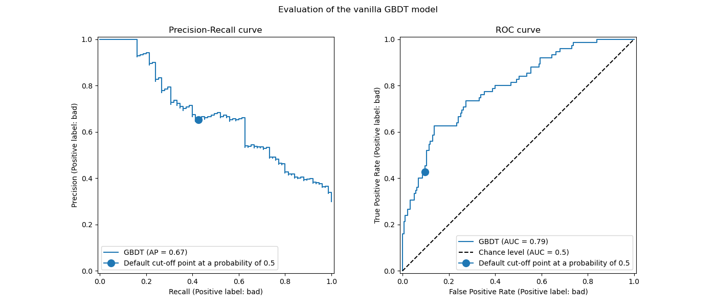
我们回顾一下,这些曲线提供了预测模型在不同截止点下的统计性能洞察。对于精确率-召回率曲线,报告的指标是精确率和召回率;对于 ROC 曲线,报告的指标是 TPR(与召回率相同)和 FPR。
在这里,不同的截止点对应于 0 到 1 之间不同级别的后验概率估计。model.predict 默认使用概率估计值 0.5 作为截止点。此截止点下的指标在曲线上用蓝色圆点表示:它对应于使用 model.predict 时模型的统计性能。
然而,我们回想一下,最初的目标是最小化成本(或最大化收益),如业务指标所定义。我们可以计算业务指标的值
print(f"Business defined metric: {scoring['credit_gain'](model, X_test, y_test)}")
Business defined metric: -232
在此阶段,我们不知道任何其他截止点是否能带来更大的收益。为了找到最优的截止点,我们需要使用业务指标计算所有可能的截止点下的成本收益,并选择最佳的。手动实现此策略可能相当繁琐,但 TunedThresholdClassifierCV 类可以帮助我们。它自动计算所有可能的截止点下的成本收益,并针对 scoring 进行优化。
调整截止点#
我们使用 TunedThresholdClassifierCV 来调整截止点。我们需要提供要优化的业务指标以及正标签。在内部,最佳截止点是通过交叉验证最大化业务指标来选择的。默认情况下,使用 5 折分层交叉验证。
from sklearn.model_selection import TunedThresholdClassifierCV

tuned_model = TunedThresholdClassifierCV(
    estimator=model,
    scoring=scoring["credit_gain"],
    store_cv_results=True,  # necessary to inspect all results
)
tuned_model.fit(X_train, y_train)
print(f"{tuned_model.best_threshold_=:0.2f}")
tuned_model.best_threshold_=0.02
我们绘制了普通模型和调优模型的 ROC 和精确召回曲线。此外,我们还绘制了每个模型将使用的截止点。由于我们稍后将重用相同的代码,因此我们定义了一个生成这些图的函数。
def plot_roc_pr_curves(vanilla_model, tuned_model, *, title):
    fig, axs = plt.subplots(nrows=1, ncols=3, figsize=(21, 6))

    linestyles = ("dashed", "dotted")
    markerstyles = ("o", ">")
    colors = ("tab:blue", "tab:orange")
    names = ("Vanilla GBDT", "Tuned GBDT")
    for idx, (est, linestyle, marker, color, name) in enumerate(
        zip((vanilla_model, tuned_model), linestyles, markerstyles, colors, names)
    ):
        decision_threshold = getattr(est, "best_threshold_", 0.5)
        PrecisionRecallDisplay.from_estimator(
            est,
            X_test,
            y_test,
            pos_label=pos_label,
            linestyle=linestyle,
            color=color,
            ax=axs[0],
            name=name,
        )
        axs[0].plot(
            scoring["recall"](est, X_test, y_test),
            scoring["precision"](est, X_test, y_test),
            marker,
            markersize=10,
            color=color,
            label=f"Cut-off point at probability of {decision_threshold:.2f}",
        )
        RocCurveDisplay.from_estimator(
            est,
            X_test,
            y_test,
            pos_label=pos_label,
            curve_kwargs=dict(linestyle=linestyle, color=color),
            ax=axs[1],
            name=name,
            plot_chance_level=idx == 1,
        )
        axs[1].plot(
            scoring["fpr"](est, X_test, y_test),
            scoring["tpr"](est, X_test, y_test),
            marker,
            markersize=10,
            color=color,
            label=f"Cut-off point at probability of {decision_threshold:.2f}",
        )

    axs[0].set_title("Precision-Recall curve")
    axs[0].legend()
    axs[1].set_title("ROC curve")
    axs[1].legend()

    axs[2].plot(
        tuned_model.cv_results_["thresholds"],
        tuned_model.cv_results_["scores"],
        color="tab:orange",
    )
    axs[2].plot(
        tuned_model.best_threshold_,
        tuned_model.best_score_,
        "o",
        markersize=10,
        color="tab:orange",
        label="Optimal cut-off point for the business metric",
    )
    axs[2].legend()
    axs[2].set_xlabel("Decision threshold (probability)")
    axs[2].set_ylabel("Objective score (using cost-matrix)")
    axs[2].set_title("Objective score as a function of the decision threshold")
    fig.suptitle(title)
title = "Comparison of the cut-off point for the vanilla and tuned GBDT model"
plot_roc_pr_curves(model, tuned_model, title=title)
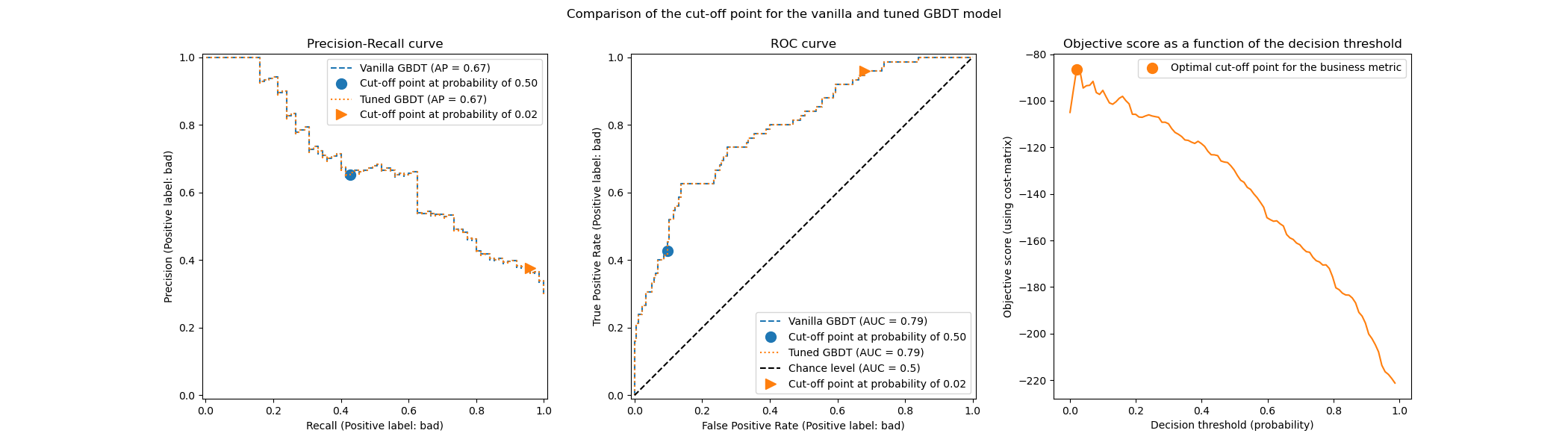
第一个值得注意的是,两个分类器具有完全相同的 ROC 和精确召回曲线。这是预料之中的,因为默认情况下,分类器是在相同的训练数据上进行拟合的。在后面的章节中,我们将更详细地讨论关于模型再拟合和交叉验证的可用选项。
第二个值得注意的是,普通模型和调优模型的截止点是不同的。为了理解为什么调优模型选择了这个截止点,我们可以查看右侧的图,该图绘制了目标分数,它与我们的业务指标完全相同。我们看到最佳阈值对应于目标分数的最大值。这个最大值是在远低于 0.5 的决策阈值下实现的:调优模型以显著降低的精确率为代价,享受了更高的召回率:调优模型更倾向于将“坏”类别标签预测给更大比例的个体。
现在我们可以检查选择这个截止点是否能在测试集上带来更好的分数。
print(f"Business defined metric: {scoring['credit_gain'](tuned_model, X_test, y_test)}")
Business defined metric: -134
我们观察到,调整决策阈值几乎将我们的业务收益提高了 2 倍。
关于模型再拟合和交叉验证的考量#
在上述实验中,我们使用了 TunedThresholdClassifierCV 的默认设置。特别是,截止点是使用 5 折分层交叉验证进行调优的。此外,一旦选择截止点,底层预测模型将在整个训练数据上重新拟合。
通过提供 refit 和 cv 参数可以更改这两种策略。例如,可以提供一个已拟合的 estimator 并设置 cv="prefit",在这种情况下,截止点将在拟合时提供的整个数据集上找到。此外,通过设置 refit=False,底层分类器不会重新拟合。在这里,我们可以尝试进行这样的实验。
model.fit(X_train, y_train)
tuned_model.set_params(cv="prefit", refit=False).fit(X_train, y_train)
print(f"{tuned_model.best_threshold_=:0.2f}")
tuned_model.best_threshold_=0.28
然后,我们以与以前相同的方法评估我们的模型
title = "Tuned GBDT model without refitting and using the entire dataset"
plot_roc_pr_curves(model, tuned_model, title=title)
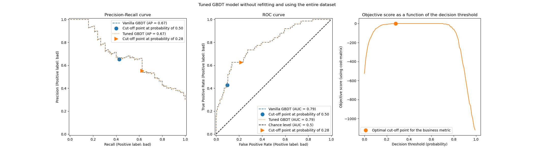
我们观察到最佳截止点与之前实验中找到的不同。如果我们查看右侧的图,我们发现业务收益在很大范围的决策阈值内有一个接近最佳 0 收益的大平台。这种行为是过拟合的症状。由于我们禁用了交叉验证,我们在模型训练的同一数据集上调整了截止点,这就是观察到过拟合的原因。
因此,应谨慎使用此选项。需要确保提供给 TunedThresholdClassifierCV 的拟合数据与用于训练底层分类器的数据不同。当只想在全新的验证集上调整预测模型而无需昂贵的完整重新拟合时,有时可能会发生这种情况。
当交叉验证成本过高时,一个潜在的替代方法是向 cv 参数提供一个介于 [0, 1] 之间的浮点数,以使用单个训练-测试拆分。它将数据拆分为训练集和测试集。让我们探讨这个选项
tuned_model.set_params(cv=0.75).fit(X_train, y_train)
title = "Tuned GBDT model without refitting and using the entire dataset"
plot_roc_pr_curves(model, tuned_model, title=title)
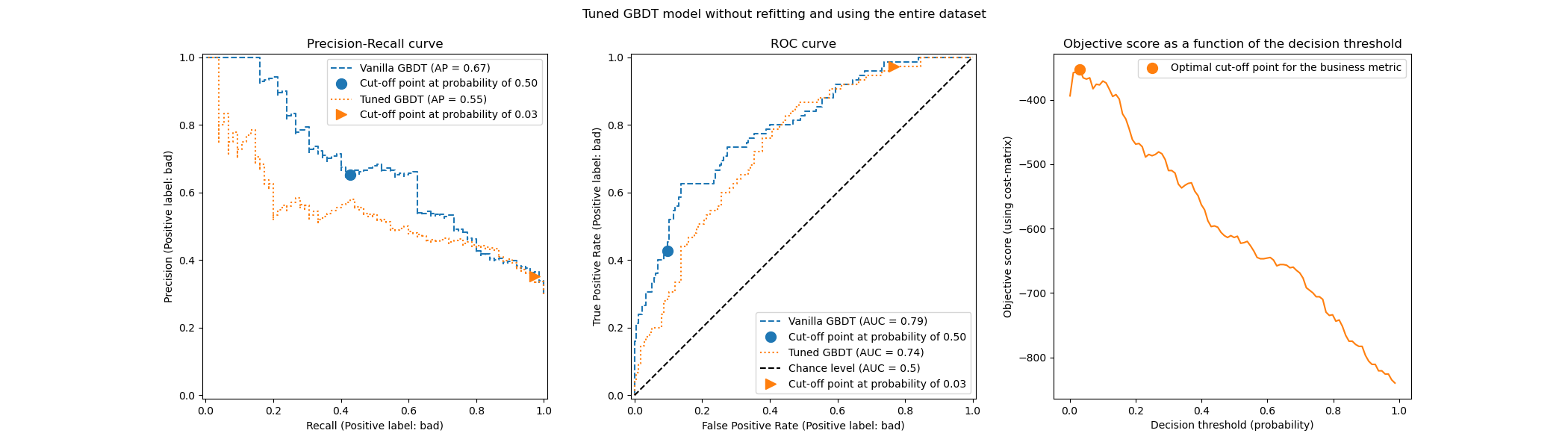
关于截止点,我们观察到其最佳值与多次重复交叉验证的情况相似。但是,请注意,单个拆分并不能解释拟合/预测过程的变异性,因此我们无法得知截止点是否存在任何方差。重复交叉验证会平均掉这种效应。
另一个观察涉及到调优模型的 ROC 和精确率-召回率曲线。正如预期的那样,这些曲线与普通模型的曲线不同,因为我们在拟合期间提供的数据子集上训练了底层分类器,并保留了一个验证集用于调优截止点。
当收益和成本不恒定时的成本敏感学习#
如 [2] 所述,在现实世界问题中,收益和成本通常不是恒定的。在本节中,我们使用与 [2] 类似的一个示例,用于信用卡交易记录中的欺诈检测问题。
信用卡数据集#
credit_card = fetch_openml(data_id=1597, as_frame=True, parser="pandas")
credit_card.frame.info()
<class 'pandas.core.frame.DataFrame'>
RangeIndex: 284807 entries, 0 to 284806
Data columns (total 30 columns):
 #   Column  Non-Null Count   Dtype
---  ------  --------------   -----
 0   V1      284807 non-null  float64
 1   V2      284807 non-null  float64
 2   V3      284807 non-null  float64
 3   V4      284807 non-null  float64
 4   V5      284807 non-null  float64
 5   V6      284807 non-null  float64
 6   V7      284807 non-null  float64
 7   V8      284807 non-null  float64
 8   V9      284807 non-null  float64
 9   V10     284807 non-null  float64
 10  V11     284807 non-null  float64
 11  V12     284807 non-null  float64
 12  V13     284807 non-null  float64
 13  V14     284807 non-null  float64
 14  V15     284807 non-null  float64
 15  V16     284807 non-null  float64
 16  V17     284807 non-null  float64
 17  V18     284807 non-null  float64
 18  V19     284807 non-null  float64
 19  V20     284807 non-null  float64
 20  V21     284807 non-null  float64
 21  V22     284807 non-null  float64
 22  V23     284807 non-null  float64
 23  V24     284807 non-null  float64
 24  V25     284807 non-null  float64
 25  V26     284807 non-null  float64
 26  V27     284807 non-null  float64
 27  V28     284807 non-null  float64
 28  Amount  284807 non-null  float64
 29  Class   284807 non-null  category
dtypes: category(1), float64(29)
memory usage: 63.3 MB
该数据集包含信用卡记录信息,其中一些是欺诈性的,另一些是合法的。因此,目标是预测信用卡记录是否为欺诈性。
columns_to_drop = ["Class"]
data = credit_card.frame.drop(columns=columns_to_drop)
target = credit_card.frame["Class"].astype(int)
首先,我们检查数据集的类别分布。
target.value_counts(normalize=True)
Class
0    0.998273
1    0.001727
Name: proportion, dtype: float64
数据集高度不平衡,欺诈交易仅占数据的 0.17%。由于我们对训练机器学习模型感兴趣,因此我们还应该确保少数类别中有足够的样本来训练模型。
target.value_counts()
Class
0    284315
1       492
Name: count, dtype: int64
我们观察到我们大约有 500 个样本,这个数量对于训练机器学习模型来说偏低。除了目标分布,我们还检查了欺诈交易金额的分布。
fraud = target == 1
amount_fraud = data["Amount"][fraud]
_, ax = plt.subplots()
ax.hist(amount_fraud, bins=30)
ax.set_title("Amount of fraud transaction")
_ = ax.set_xlabel("Amount (€)")
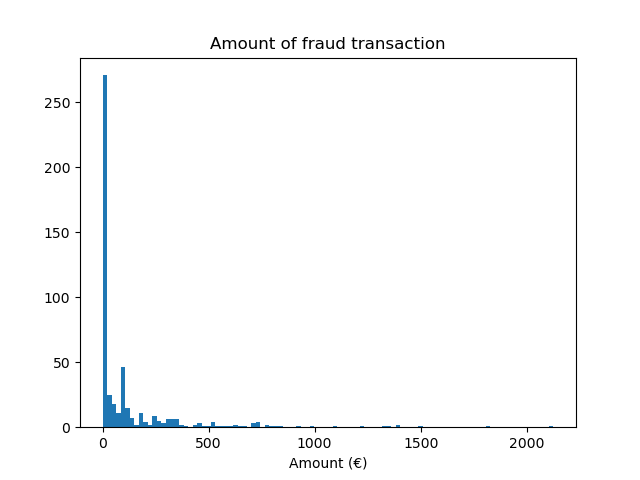
使用业务指标解决问题#
现在,我们创建了依赖于每笔交易金额的业务指标。我们像 [2] 中一样定义成本矩阵。接受合法交易可获得交易金额 2% 的收益。然而,接受欺诈交易会导致交易金额的损失。如 [2] 所述,与拒绝(欺诈和合法交易)相关的收益和损失很难定义。在这里,我们定义拒绝合法交易估计损失 5 欧元,而拒绝欺诈交易估计收益 50 欧元。因此,我们定义以下函数来计算给定决策的总收益
def business_metric(y_true, y_pred, amount):
    mask_true_positive = (y_true == 1) & (y_pred == 1)
    mask_true_negative = (y_true == 0) & (y_pred == 0)
    mask_false_positive = (y_true == 0) & (y_pred == 1)
    mask_false_negative = (y_true == 1) & (y_pred == 0)
    fraudulent_refuse = mask_true_positive.sum() * 50
    fraudulent_accept = -amount[mask_false_negative].sum()
    legitimate_refuse = mask_false_positive.sum() * -5
    legitimate_accept = (amount[mask_true_negative] * 0.02).sum()
    return fraudulent_refuse + fraudulent_accept + legitimate_refuse + legitimate_accept
基于此业务指标,我们创建一个 scikit-learn 评分器,该评分器在给定拟合分类器和测试集的情况下计算业务指标。为此,我们使用 make_scorer 工厂。变量 amount 是要传递给评分器的额外元数据,我们需要使用 元数据路由 来考虑此信息。
sklearn.set_config(enable_metadata_routing=True)
business_scorer = make_scorer(business_metric).set_score_request(amount=True)
因此,在这个阶段,我们观察到交易金额被使用了两次:一次作为训练预测模型的特征,一次作为元数据来计算业务指标,从而计算模型的统计性能。当作为特征使用时,我们只需要在 data 中有一个包含每笔交易金额的列。要将此信息用作元数据,我们需要有一个外部变量,我们可以将其传递给评分器或模型,该模型会在内部将此元数据路由到评分器。所以让我们创建这个变量。
amount = credit_card.frame["Amount"].to_numpy()
from sklearn.model_selection import train_test_split

data_train, data_test, target_train, target_test, amount_train, amount_test = (
    train_test_split(
        data, target, amount, stratify=target, test_size=0.5, random_state=42
    )
)
我们首先评估一些基线策略作为参考。回想一下,类别“0”是合法类别,类别“1”是欺诈类别。
from sklearn.dummy import DummyClassifier

always_accept_policy = DummyClassifier(strategy="constant", constant=0)
always_accept_policy.fit(data_train, target_train)
benefit = business_scorer(
    always_accept_policy, data_test, target_test, amount=amount_test
)
print(f"Benefit of the 'always accept' policy: {benefit:,.2f}€")
Benefit of the 'always accept' policy: 221,445.07€
将所有交易视为合法的策略将创造约 220,000 欧元的利润。我们对预测所有交易均为欺诈的分类器进行相同的评估。
always_reject_policy = DummyClassifier(strategy="constant", constant=1)
always_reject_policy.fit(data_train, target_train)
benefit = business_scorer(
    always_reject_policy, data_test, target_test, amount=amount_test
)
print(f"Benefit of the 'always reject' policy: {benefit:,.2f}€")
Benefit of the 'always reject' policy: -698,490.00€
这样的政策将导致灾难性的损失:约 670,000 欧元。这是意料之中的,因为绝大多数交易都是合法的,而该政策将以不菲的成本拒绝它们。
理想情况下,一个根据每笔交易情况调整接受/拒绝决策的预测模型,应该能让我们获得比我们最佳的恒定基线策略 220,000 欧元更高的利润。
我们从一个默认决策阈值为 0.5 的逻辑回归模型开始。在这里,我们使用适当的评分规则(对数损失)调整逻辑回归的超参数 C,以确保模型通过其 predict_proba 方法返回的概率预测尽可能准确,而与决策阈值的选择无关。
from sklearn.linear_model import LogisticRegression
from sklearn.model_selection import GridSearchCV
from sklearn.pipeline import make_pipeline
from sklearn.preprocessing import StandardScaler

logistic_regression = make_pipeline(StandardScaler(), LogisticRegression())
param_grid = {"logisticregression__C": np.logspace(-6, 6, 13)}
model = GridSearchCV(logistic_regression, param_grid, scoring="neg_log_loss").fit(
    data_train, target_train
)
model
调整决策阈值#
现在的问题是:我们的模型是否针对我们想要进行的决策类型进行了优化?到目前为止,我们尚未优化决策阈值。我们使用 TunedThresholdClassifierCV 来优化给定业务评分器的决策。为了避免嵌套交叉验证,我们将使用前一次网格搜索中找到的最佳估计器。
tuned_model = TunedThresholdClassifierCV(
    estimator=model.best_estimator_,
    scoring=business_scorer,
    thresholds=100,
    n_jobs=2,
)
由于我们的业务评分器需要每笔交易的金额,因此我们需要在 fit 方法中传递此信息。TunedThresholdClassifierCV 负责自动将此元数据分派给底层评分器。
tuned_model.fit(data_train, target_train, amount=amount_train)
手动设置决策阈值而不是调整它#
在前面的示例中,我们使用 TunedThresholdClassifierCV 来找到最佳决策阈值。然而,在某些情况下,我们可能对手头的问题有一些先验知识,并且可能乐于手动设置决策阈值。
类 FixedThresholdClassifier 允许我们手动设置决策阈值。在预测时,它的行为与之前调整过的模型相同,但在拟合过程中不进行任何搜索。请注意,这里我们使用 FrozenEstimator 来包装预测模型,以避免任何重新拟合。
这里,我们将重用上一节中找到的决策阈值来创建一个新模型,并检查它是否给出相同的结果。
from sklearn.frozen import FrozenEstimator
from sklearn.model_selection import FixedThresholdClassifier

model_fixed_threshold = FixedThresholdClassifier(
    estimator=FrozenEstimator(model), threshold=tuned_model.best_threshold_
)
business_score = business_scorer(
    model_fixed_threshold, data_test, target_test, amount=amount_test
)
print(f"Benefit of logistic regression with a tuned threshold:  {business_score:,.2f}€")
Benefit of logistic regression with a tuned threshold: 249,433.39€
我们观察到我们得到了完全相同的结果,但拟合过程要快得多,因为我们没有执行任何超参数搜索。
最后,业务指标的(平均)估计值本身可能不可靠,特别是在少数类别的数据点数量非常少时。通过对历史数据(离线评估)进行业务指标交叉验证估计的任何业务影响,理想情况下都应通过对实时数据(在线评估)进行 A/B 测试来确认。但请注意,A/B 测试模型超出了 scikit-learn 库本身的范围。
最后,我们禁用元数据路由的配置标志
.. GENERATED FROM PYTHON SOURCE LINES 694-695
sklearn.set_config(enable_metadata_routing=False)
脚本总运行时间: (0 分钟 35.875 秒)
相关示例