使用多项式核近似的可扩展学习#

本示例展示了如何使用 PolynomialCountSketch 高效生成多项式核特征空间近似。该方法用于训练能够近似核方法分类准确率的线性分类器。

我们使用 Covtype 数据集 [2]，尝试复现 Tensor Sketch 原始论文 [1] 中的实验，即 PolynomialCountSketch 所实现的算法。

首先，我们计算线性分类器在原始特征上的准确率。然后，我们针对 PolynomialCountSketch 生成的不同数量的特征（n_components）训练线性分类器，从而以可扩展的方式近似核分类器的准确率。

# Authors: The scikit-learn developers
# SPDX-License-Identifier: BSD-3-Clause

准备数据#

加载 Covtype 数据集，该数据集包含 581,012 个样本，每个样本有 54 个特征，分布在 6 个类别中。该数据集的目标是仅通过测绘变量（无遥感数据）来预测森林覆盖类型。加载后，我们将其转换为二分类问题，以匹配 LIBSVM 网页 [2] 上的数据集版本，这也是 [1] 中所使用的版本。

from sklearn.datasets import fetch_covtype

X, y = fetch_covtype(return_X_y=True)

y[y != 2] = 0
y[y == 2] = 1  # We will try to separate class 2 from the other 6 classes.

数据划分#

在这里，我们选择 5,000 个样本进行训练，10,000 个用于测试。若要完全复现原始 Tensor Sketch 论文中的结果，请选择 100,000 个样本进行训练。

from sklearn.model_selection import train_test_split

X_train, X_test, y_train, y_test = train_test_split(
    X, y, train_size=5_000, test_size=10_000, random_state=42
)

特征归一化#

现在将特征缩放到 [0, 1] 范围，以匹配 LIBSVM 网页上的数据集格式，然后按照原始 Tensor Sketch 论文 [1] 的做法将其归一化为单位长度。

from sklearn.pipeline import make_pipeline
from sklearn.preprocessing import MinMaxScaler, Normalizer

mm = make_pipeline(MinMaxScaler(), Normalizer())
X_train = mm.fit_transform(X_train)
X_test = mm.transform(X_test)

建立基准模型#

作为基准，在原始特征上训练一个线性 SVM 并打印其准确率。我们还测量并存储准确率和训练时间，以便稍后绘图。

import time

from sklearn.svm import LinearSVC

results = {}

lsvm = LinearSVC()
start = time.time()
lsvm.fit(X_train, y_train)
lsvm_time = time.time() - start
lsvm_score = 100 * lsvm.score(X_test, y_test)

results["LSVM"] = {"time": lsvm_time, "score": lsvm_score}
print(f"Linear SVM score on raw features: {lsvm_score:.2f}%")

Linear SVM score on raw features: 75.62%

建立核近似模型#

随后，我们使用 PolynomialCountSketch 生成的不同 n_components 值的特征来训练线性 SVM，结果表明这些核特征近似提高了线性分类的准确率。在典型应用场景中，为了获得相对于线性分类的性能提升，n_components 的值应大于输入表示中的特征数量。经验法则显示，评估得分/运行时间成本的最优值通常在 n_components = 10 * n_features 左右达到，但这取决于具体处理的数据集。请注意，由于原始样本有 54 个特征，四次多项式核的显式特征映射将拥有约 850 万个特征（准确地说是 54^4）。多亏了 PolynomialCountSketch，我们可以将该特征空间中大部分判别信息浓缩为一个极其紧凑的表示。虽然在本示例中我们只运行了一次实验（n_runs = 1），但在实践中，应当多次重复实验以弥补 PolynomialCountSketch 的随机性。

from sklearn.kernel_approximation import PolynomialCountSketch

n_runs = 1
N_COMPONENTS = [250, 500, 1000, 2000]

for n_components in N_COMPONENTS:
    ps_lsvm_time = 0
    ps_lsvm_score = 0
    for _ in range(n_runs):
        pipeline = make_pipeline(
            PolynomialCountSketch(n_components=n_components, degree=4),
            LinearSVC(),
        )

        start = time.time()
        pipeline.fit(X_train, y_train)
        ps_lsvm_time += time.time() - start
        ps_lsvm_score += 100 * pipeline.score(X_test, y_test)

    ps_lsvm_time /= n_runs
    ps_lsvm_score /= n_runs

    results[f"LSVM + PS({n_components})"] = {
        "time": ps_lsvm_time,
        "score": ps_lsvm_score,
    }
    print(
        f"Linear SVM score on {n_components} PolynomialCountSketch "
        f"features: {ps_lsvm_score:.2f}%"
    )

Linear SVM score on 250 PolynomialCountSketch features: 76.22%
Linear SVM score on 500 PolynomialCountSketch features: 77.60%
Linear SVM score on 1000 PolynomialCountSketch features: 77.75%
Linear SVM score on 2000 PolynomialCountSketch features: 78.26%

建立核 SVM 模型#

训练一个核 SVM，以观察 PolynomialCountSketch 在多大程度上近似了核方法的性能。当然，这可能需要一些时间，因为 SVC 类（支持向量分类器）的可扩展性相对较差。这就是为什么核近似方法如此有用的原因。

from sklearn.svm import SVC

ksvm = SVC(C=500.0, kernel="poly", degree=4, coef0=0, gamma=1.0)

start = time.time()
ksvm.fit(X_train, y_train)
ksvm_time = time.time() - start
ksvm_score = 100 * ksvm.score(X_test, y_test)

results["KSVM"] = {"time": ksvm_time, "score": ksvm_score}
print(f"Kernel-SVM score on raw features: {ksvm_score:.2f}%")

Kernel-SVM score on raw features: 79.78%

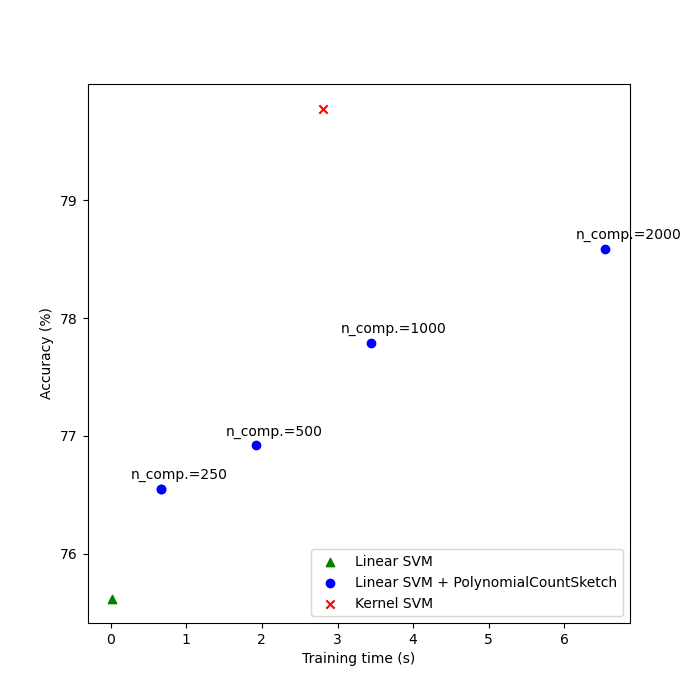
结果比较#

最后，绘制不同方法的准确率与训练时间的关系图。正如我们所见，核 SVM 虽然达到了更高的准确率，但其训练时间要长得多，且最重要的是，如果训练样本数量增加，其训练时间增长得会更快。

import matplotlib.pyplot as plt

fig, ax = plt.subplots(figsize=(7, 7))
ax.scatter(
    [
        results["LSVM"]["time"],
    ],
    [
        results["LSVM"]["score"],
    ],
    label="Linear SVM",
    c="green",
    marker="^",
)

ax.scatter(
    [
        results["LSVM + PS(250)"]["time"],
    ],
    [
        results["LSVM + PS(250)"]["score"],
    ],
    label="Linear SVM + PolynomialCountSketch",
    c="blue",
)

for n_components in N_COMPONENTS:
    ax.scatter(
        [
            results[f"LSVM + PS({n_components})"]["time"],
        ],
        [
            results[f"LSVM + PS({n_components})"]["score"],
        ],
        c="blue",
    )
    ax.annotate(
        f"n_comp.={n_components}",
        (
            results[f"LSVM + PS({n_components})"]["time"],
            results[f"LSVM + PS({n_components})"]["score"],
        ),
        xytext=(-30, 10),
        textcoords="offset pixels",
    )

ax.scatter(
    [
        results["KSVM"]["time"],
    ],
    [
        results["KSVM"]["score"],
    ],
    label="Kernel SVM",
    c="red",
    marker="x",
)

ax.set_xlabel("Training time (s)")
ax.set_ylabel("Accuracy (%)")
ax.legend()
plt.show()

参考文献#

脚本总运行时间： (0 分钟 20.253 秒)