注意
转到末尾以下载完整示例代码或通过 JupyterLite 或 Binder 在浏览器中运行此示例。
三分类问题的概率校准#
此示例说明了 sigmoid 校准如何改变三分类问题的预测概率。图示为标准的2-单纯形(2-simplex),其中三个角对应于三个类别。箭头从未校准分类器预测的概率向量指向同一分类器在保留验证集上经过 sigmoid 校准后预测的概率向量。颜色表示实例的真实类别(红色:类别1,绿色:类别2,蓝色:类别3)。
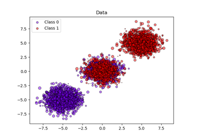
数据#
下面,我们生成一个包含2000个样本、2个特征和3个目标类别(target classes)的分类数据集。然后我们按如下方式拆分数据:
训练集:600个样本(用于训练分类器)
验证集:400个样本(用于校准预测概率)
测试集:1000个样本
注意,我们还创建了 X_train_valid 和 y_train_valid,它们包含训练集和验证集的子集。当只希望训练分类器而不校准预测概率时,会使用这些数据。
# Authors: The scikit-learn developers
# SPDX-License-Identifier: BSD-3-Clause

import numpy as np

from sklearn.datasets import make_blobs

np.random.seed(0)

X, y = make_blobs(
    n_samples=2000, n_features=2, centers=3, random_state=42, cluster_std=5.0
)
X_train, y_train = X[:600], y[:600]
X_valid, y_valid = X[600:1000], y[600:1000]
X_train_valid, y_train_valid = X[:1000], y[:1000]
X_test, y_test = X[1000:], y[1000:]
拟合与校准#
首先,我们将在串联的训练集和验证集数据(1000个样本)上训练一个包含25个基本估计器(树)的 RandomForestClassifier。这是未校准的分类器。
from sklearn.ensemble import RandomForestClassifier

clf = RandomForestClassifier(n_estimators=25)
clf.fit(X_train_valid, y_train_valid)
为了训练校准后的分类器,我们从相同的 RandomForestClassifier 开始,但仅使用训练数据子集(600个样本)进行训练,然后使用验证数据子集(400个样本)以两阶段过程进行校准,其中 method='sigmoid'。
from sklearn.calibration import CalibratedClassifierCV
from sklearn.frozen import FrozenEstimator

clf = RandomForestClassifier(n_estimators=25)
clf.fit(X_train, y_train)
cal_clf = CalibratedClassifierCV(FrozenEstimator(clf), method="sigmoid")
cal_clf.fit(X_valid, y_valid)
比较概率#
下面我们绘制一个2-单纯形,其中的箭头显示了测试样本预测概率的变化。
import matplotlib.pyplot as plt

plt.figure(figsize=(10, 10))
colors = ["r", "g", "b"]

clf_probs = clf.predict_proba(X_test)
cal_clf_probs = cal_clf.predict_proba(X_test)
# Plot arrows
for i in range(clf_probs.shape[0]):
    plt.arrow(
        clf_probs[i, 0],
        clf_probs[i, 1],
        cal_clf_probs[i, 0] - clf_probs[i, 0],
        cal_clf_probs[i, 1] - clf_probs[i, 1],
        color=colors[y_test[i]],
        head_width=1e-2,
    )

# Plot perfect predictions, at each vertex
plt.plot([1.0], [0.0], "ro", ms=20, label="Class 1")
plt.plot([0.0], [1.0], "go", ms=20, label="Class 2")
plt.plot([0.0], [0.0], "bo", ms=20, label="Class 3")

# Plot boundaries of unit simplex
plt.plot([0.0, 1.0, 0.0, 0.0], [0.0, 0.0, 1.0, 0.0], "k", label="Simplex")

# Annotate points 6 points around the simplex, and mid point inside simplex
plt.annotate(
    r"($\frac{1}{3}$, $\frac{1}{3}$, $\frac{1}{3}$)",
    xy=(1.0 / 3, 1.0 / 3),
    xytext=(1.0 / 3, 0.23),
    xycoords="data",
    arrowprops=dict(facecolor="black", shrink=0.05),
    horizontalalignment="center",
    verticalalignment="center",
)
plt.plot([1.0 / 3], [1.0 / 3], "ko", ms=5)
plt.annotate(
    r"($\frac{1}{2}$, $0$, $\frac{1}{2}$)",
    xy=(0.5, 0.0),
    xytext=(0.5, 0.1),
    xycoords="data",
    arrowprops=dict(facecolor="black", shrink=0.05),
    horizontalalignment="center",
    verticalalignment="center",
)
plt.annotate(
    r"($0$, $\frac{1}{2}$, $\frac{1}{2}$)",
    xy=(0.0, 0.5),
    xytext=(0.1, 0.5),
    xycoords="data",
    arrowprops=dict(facecolor="black", shrink=0.05),
    horizontalalignment="center",
    verticalalignment="center",
)
plt.annotate(
    r"($\frac{1}{2}$, $\frac{1}{2}$, $0$)",
    xy=(0.5, 0.5),
    xytext=(0.6, 0.6),
    xycoords="data",
    arrowprops=dict(facecolor="black", shrink=0.05),
    horizontalalignment="center",
    verticalalignment="center",
)
plt.annotate(
    r"($0$, $0$, $1$)",
    xy=(0, 0),
    xytext=(0.1, 0.1),
    xycoords="data",
    arrowprops=dict(facecolor="black", shrink=0.05),
    horizontalalignment="center",
    verticalalignment="center",
)
plt.annotate(
    r"($1$, $0$, $0$)",
    xy=(1, 0),
    xytext=(1, 0.1),
    xycoords="data",
    arrowprops=dict(facecolor="black", shrink=0.05),
    horizontalalignment="center",
    verticalalignment="center",
)
plt.annotate(
    r"($0$, $1$, $0$)",
    xy=(0, 1),
    xytext=(0.1, 1),
    xycoords="data",
    arrowprops=dict(facecolor="black", shrink=0.05),
    horizontalalignment="center",
    verticalalignment="center",
)
# Add grid
plt.grid(False)
for x in [0.0, 0.1, 0.2, 0.3, 0.4, 0.5, 0.6, 0.7, 0.8, 0.9, 1.0]:
    plt.plot([0, x], [x, 0], "k", alpha=0.2)
    plt.plot([0, 0 + (1 - x) / 2], [x, x + (1 - x) / 2], "k", alpha=0.2)
    plt.plot([x, x + (1 - x) / 2], [0, 0 + (1 - x) / 2], "k", alpha=0.2)

plt.title("Change of predicted probabilities on test samples after sigmoid calibration")
plt.xlabel("Probability class 1")
plt.ylabel("Probability class 2")
plt.xlim(-0.05, 1.05)
plt.ylim(-0.05, 1.05)
_ = plt.legend(loc="best")
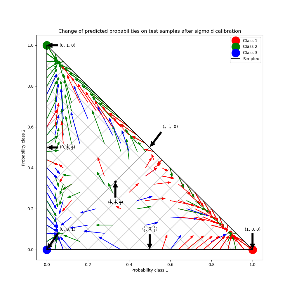
在上图中,单纯形的每个顶点代表一个完美预测的类别(例如,1, 0, 0)。单纯形内部的中点代表预测三个类别的概率相等(即 1/3, 1/3, 1/3)。每个箭头从未校准的概率开始,箭头头部指向校准后的概率。箭头的颜色代表该测试样本的真实类别。
未校准的分类器对其预测过于自信,并产生较大的 对数损失。校准后的分类器产生较低的 对数损失,原因有两个。首先,请注意上图中箭头通常指向远离单纯形边缘的方向,在边缘处某个类别的概率为0。其次,大部分箭头指向真实类别,例如,绿色箭头(真实类别为“绿色”的样本)通常指向绿色顶点。这导致更少的过于自信、预测概率为0的情况,同时增加了正确类别的预测概率。因此,校准后的分类器产生更准确的预测概率,从而产生较低的 对数损失。
我们可以通过比较未校准和校准分类器在1000个测试样本上的预测的 对数损失 来客观地证明这一点。请注意,另一种选择是增加 RandomForestClassifier 的基本估计器(树)数量,这也会导致类似的 对数损失 降低。
Log-loss of:
 - uncalibrated classifier: 1.327
 - calibrated classifier: 0.549
我们还可以使用 Brier score 来评估概率预测的校准情况(越低越好,范围为 [0, 2])
from sklearn.metrics import brier_score_loss

loss = brier_score_loss(y_test, clf_probs)
cal_loss = brier_score_loss(y_test, cal_clf_probs)

print("Brier score of")
print(f" - uncalibrated classifier: {loss:.3f}")
print(f" - calibrated classifier: {cal_loss:.3f}")
Brier score of
 - uncalibrated classifier: 0.308
 - calibrated classifier: 0.310
根据 Brier score,校准后的分类器并不优于原始模型。
最后,我们生成一个2-单纯形上可能的未校准概率网格,计算相应的校准概率,并为每个点绘制箭头。箭头根据最高的未校准概率着色。这说明了学习到的校准映射。
plt.figure(figsize=(10, 10))
# Generate grid of probability values
p1d = np.linspace(0, 1, 20)
p0, p1 = np.meshgrid(p1d, p1d)
p2 = 1 - p0 - p1
p = np.c_[p0.ravel(), p1.ravel(), p2.ravel()]
p = p[p[:, 2] >= 0]

# Use the three class-wise calibrators to compute calibrated probabilities
calibrated_classifier = cal_clf.calibrated_classifiers_[0]
prediction = np.vstack(
    [
        calibrator.predict(this_p)
        for calibrator, this_p in zip(calibrated_classifier.calibrators, p.T)
    ]
).T

# Re-normalize the calibrated predictions to make sure they stay inside the
# simplex. This same renormalization step is performed internally by the
# predict method of CalibratedClassifierCV on multiclass problems.
prediction /= prediction.sum(axis=1)[:, None]

# Plot changes in predicted probabilities induced by the calibrators
for i in range(prediction.shape[0]):
    plt.arrow(
        p[i, 0],
        p[i, 1],
        prediction[i, 0] - p[i, 0],
        prediction[i, 1] - p[i, 1],
        head_width=1e-2,
        color=colors[np.argmax(p[i])],
    )

# Plot the boundaries of the unit simplex
plt.plot([0.0, 1.0, 0.0, 0.0], [0.0, 0.0, 1.0, 0.0], "k", label="Simplex")

plt.grid(False)
for x in [0.0, 0.1, 0.2, 0.3, 0.4, 0.5, 0.6, 0.7, 0.8, 0.9, 1.0]:
    plt.plot([0, x], [x, 0], "k", alpha=0.2)
    plt.plot([0, 0 + (1 - x) / 2], [x, x + (1 - x) / 2], "k", alpha=0.2)
    plt.plot([x, x + (1 - x) / 2], [0, 0 + (1 - x) / 2], "k", alpha=0.2)

plt.title("Learned sigmoid calibration map")
plt.xlabel("Probability class 1")
plt.ylabel("Probability class 2")
plt.xlim(-0.05, 1.05)
plt.ylim(-0.05, 1.05)

plt.show()
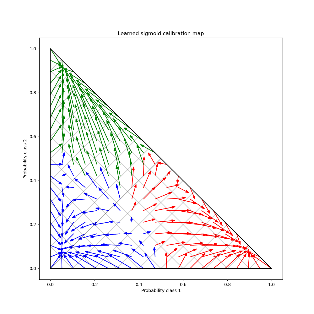
可以观察到,平均而言,校准器将高度自信的预测推离单纯形的边界,同时将不确定的预测推向三个模式之一,每个模式对应一个类别。我们还可以观察到映射不是对称的。此外,一些箭头似乎跨越了类别分配边界,这不一定是人们期望从校准映射中看到的,因为它意味着一些预测类别在校准后会发生变化。
总而言之,不应盲目信任 CalibratedClassifierCV 中实现的一对多(One-vs-Rest)多类别校准策略。
脚本总运行时间: (0 minutes 1.214 seconds)
相关示例