注意
转到末尾 下载完整的示例代码或通过 JupyterLite 或 Binder 在浏览器中运行此示例。
半监督分类器与 SVM 在 Iris 数据集上的决策边界#
此示例比较了两种半监督方法学习到的决策边界,即 LabelSpreading 和 SelfTrainingClassifier,同时改变标记训练数据的比例,从很小的比例到整个数据集。
这两种方法都依赖于 RBF 核:LabelSpreading 默认使用它,而 SelfTrainingClassifier 在这里与 SVC 作为基础估计器配对(默认也基于 RBF),以进行公平比较。当有 100% 标记数据时,SelfTrainingClassifier 简化为完全监督的 SVC,因为没有未标记的点可以进行伪标记。
在第二部分中,我们解释了 LabelSpreading 和 SelfTrainingClassifier 中 predict_proba 是如何计算的。
请参阅 文本数据集上的半监督分类,了解 LabelSpreading 和 SelfTrainingClassifier 在性能方面的比较。
# Authors: The scikit-learn developers
# SPDX-License-Identifier: BSD-3-Clause
import matplotlib.patches as mpatches
import matplotlib.pyplot as plt
import numpy as np

from sklearn.datasets import load_iris
from sklearn.inspection import DecisionBoundaryDisplay
from sklearn.semi_supervised import LabelSpreading, SelfTrainingClassifier
from sklearn.svm import SVC

iris = load_iris()
X = iris.data[:, :2]
y = iris.target

rng = np.random.RandomState(42)
y_rand = rng.rand(y.shape[0])
y_10 = np.copy(y)
y_10[y_rand > 0.1] = -1  # set random samples to be unlabeled
y_30 = np.copy(y)
y_30[y_rand > 0.3] = -1

ls10 = (LabelSpreading().fit(X, y_10), y_10, "LabelSpreading with 10% labeled data")
ls30 = (LabelSpreading().fit(X, y_30), y_30, "LabelSpreading with 30% labeled data")
ls100 = (LabelSpreading().fit(X, y), y, "LabelSpreading with 100% labeled data")

base_classifier = SVC(gamma=0.5, probability=True, random_state=42)
st10 = (
    SelfTrainingClassifier(base_classifier).fit(X, y_10),
    y_10,
    "Self-training with 10% labeled data",
)
st30 = (
    SelfTrainingClassifier(base_classifier).fit(X, y_30),
    y_30,
    "Self-training with 30% labeled data",
)
rbf_svc = (
    base_classifier.fit(X, y),
    y,
    "SVC with rbf kernel\n(equivalent to Self-training with 100% labeled data)",
)

tab10 = plt.get_cmap("tab10")
color_map = {cls: tab10(cls) for cls in np.unique(y)}
color_map[-1] = (1, 1, 1)
classifiers = (ls10, st10, ls30, st30, ls100, rbf_svc)

fig, axes = plt.subplots(nrows=3, ncols=2, sharex="col", sharey="row", figsize=(10, 12))
axes = axes.ravel()

handles = [
    mpatches.Patch(facecolor=tab10(i), edgecolor="black", label=iris.target_names[i])
    for i in np.unique(y)
]
handles.append(mpatches.Patch(facecolor="white", edgecolor="black", label="Unlabeled"))

for ax, (clf, y_train, title) in zip(axes, classifiers):
    DecisionBoundaryDisplay.from_estimator(
        clf,
        X,
        response_method="predict_proba",
        plot_method="contourf",
        ax=ax,
    )
    colors = [color_map[label] for label in y_train]
    ax.scatter(X[:, 0], X[:, 1], c=colors, edgecolor="black")
    ax.set_title(title)
fig.suptitle(
    "Semi-supervised decision boundaries with varying fractions of labeled data", y=1
)
fig.legend(
    handles=handles, loc="lower center", ncol=len(handles), bbox_to_anchor=(0.5, 0.0)
)
fig.tight_layout(rect=[0, 0.03, 1, 1])
plt.show()
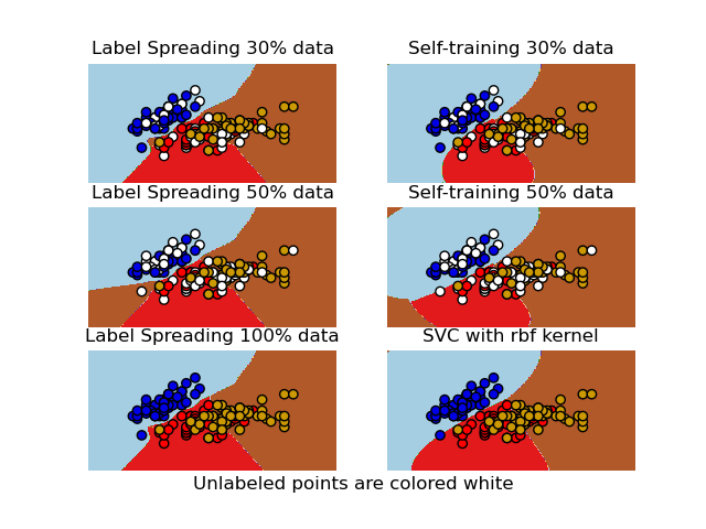
我们观察到,即使只使用了非常小一部分的标签,决策边界也已经与使用所有可用标记数据进行训练的决策边界非常相似。
predict_proba 的解释#
LabelSpreading 中的 predict_proba#
LabelSpreading 从数据中构建一个相似性图,默认使用 RBF 核。这意味着每个样本都与所有其他样本连接,连接权重随着它们平方欧几里得距离的增加而衰减,并由参数 gamma 进行缩放。
一旦有了这个加权图,标签就会沿着图的边传播。每个样本逐渐接受一个反映其邻居标签加权平均值的软标签分布,直到过程收敛。这些每个样本的分布存储在 label_distributions_ 中。
predict_proba 通过对 label_distributions_ 中的行进行加权平均来计算新点的类别概率,其中权重来自新点与训练样本之间的 RBF 核相似性。然后对平均值进行重新归一化,使其总和为一。
请记住,这些“概率”是基于图的分数,而不是经过校准的后验概率。不要过分解释它们的绝对值。
from sklearn.metrics.pairwise import rbf_kernel

ls = ls100[0]  # fitted LabelSpreading instance
x_query = np.array([[3.5, 1.5]])  # point in the soft blue region

# Step 1: similarities between query and all training samples
W = rbf_kernel(x_query, X, gamma=ls.gamma)  # `gamma=20` by default

# Step 2: weighted average of label distributions
probs = np.dot(W, ls.label_distributions_)

# Step 3: normalize to sum to 1
probs /= probs.sum(axis=1, keepdims=True)

print("Manual:", probs)
print("API   :", ls.predict_proba(x_query))
Manual: [[0.96 0.03 0.01]]
API   : [[0.96 0.03 0.01]]
SelfTrainingClassifier 中的 predict_proba#
SelfTrainingClassifier 的工作原理是:重复地在当前标记的数据上拟合其基础估计器,然后为预测概率超过置信度阈值的未标记点添加伪标签。这个过程一直持续到没有新的点可以被标记为止,此时分类器有一个最终拟合的基础估计器存储在属性 estimator_ 中。
当你对 SelfTrainingClassifier 调用 predict_proba 时,它只是委托给这个最终的估计器。
st = st10[0]
print("Manual:", st.estimator_.predict_proba(x_query))
print("API   :", st.predict_proba(x_query))
Manual: [[0.52 0.29 0.19]]
API   : [[0.52 0.29 0.19]]
在这两种方法中,半监督学习可以理解为为每个样本构建一个关于类别的分类分布。LabelSpreading 保持这些分布是软性的,并通过基于图的传播进行更新。预测(包括 predict_proba)仍然与训练集相关联,必须存储训练集才能进行推断。
SelfTrainingClassifier 则在训练期间内部使用这些分布来决定哪些未标记点要分配伪标签,但在预测时返回的概率直接来自最终拟合的估计器,因此决策规则不需要存储训练数据。
脚本总运行时间: (0 分钟 0.818 秒)
相关示例