注意
转到末尾 以下载完整示例代码,或通过 JupyterLite 或 Binder 在浏览器中运行此示例
决策函数的决策阈值事后调优#
二分类器训练完成后,predict 方法会输出类别标签预测,这些预测是通过对 decision_function 或 predict_proba 输出进行阈值处理得到的。默认阈值定义为 0.5 的后验概率估计或 0.0 的决策分数。然而,这种默认策略可能不适用于手头的任务。
本示例展示了如何使用 TunedThresholdClassifierCV 根据感兴趣的度量标准来调整决策阈值。
# Authors: The scikit-learn developers
# SPDX-License-Identifier: BSD-3-Clause
糖尿病数据集#
为了说明决策阈值的调整,我们将使用糖尿病数据集。该数据集可在 OpenML 上获取:https://www.openml.org/d/37。我们使用 fetch_openml 函数来获取此数据集。
from sklearn.datasets import fetch_openml

diabetes = fetch_openml(data_id=37, as_frame=True, parser="pandas")
data, target = diabetes.data, diabetes.target
我们查看目标变量以了解我们正在处理的问题类型。
target.value_counts()
class
tested_negative    500
tested_positive    268
Name: count, dtype: int64
我们可以看到我们正在处理一个二分类问题。由于标签未编码为 0 和 1,我们明确指出将标签为“tested_negative”的类别视为负类别(这也是最常见的类别),将标签为“tested_positive”的类别视为正类别
neg_label, pos_label = target.value_counts().index
我们还可以观察到,这个二分类问题略微不平衡,负类别的样本数量大约是正类别的两倍。在评估时,我们应该考虑这一方面来解释结果。
我们的基础分类器#
我们定义了一个由缩放器和逻辑回归分类器组成的基础预测模型。
from sklearn.linear_model import LogisticRegression
from sklearn.pipeline import make_pipeline
from sklearn.preprocessing import StandardScaler

model = make_pipeline(StandardScaler(), LogisticRegression())
model
我们使用交叉验证来评估模型。我们使用准确率和平衡准确率来报告模型的性能。平衡准确率是一种对类别不平衡不那么敏感的度量标准,它将帮助我们更全面地看待准确率分数。
交叉验证使我们能够研究决策阈值在数据不同分割上的方差。然而,数据集相当小,使用超过 5 折来评估离散度将是有害的。因此,我们使用 RepeatedStratifiedKFold,其中我们应用多次 5 折交叉验证。
import pandas as pd

from sklearn.model_selection import RepeatedStratifiedKFold, cross_validate

scoring = ["accuracy", "balanced_accuracy"]
cv_scores = [
    "train_accuracy",
    "test_accuracy",
    "train_balanced_accuracy",
    "test_balanced_accuracy",
]
cv = RepeatedStratifiedKFold(n_splits=5, n_repeats=10, random_state=42)
cv_results_vanilla_model = pd.DataFrame(
    cross_validate(
        model,
        data,
        target,
        scoring=scoring,
        cv=cv,
        return_train_score=True,
        return_estimator=True,
    )
)
cv_results_vanilla_model[cv_scores].aggregate(["mean", "std"]).T
我们的预测模型成功地把握了数据和目标之间的关系。训练和测试分数彼此接近,这意味着我们的预测模型没有过拟合。我们还可以观察到,由于前面提到的类别不平衡,平衡准确率低于准确率。
对于这个分类器,我们将用于将正类别概率转换为类别预测的决策阈值设置为其默认值:0.5。然而,这个阈值可能不是最优的。如果我们感兴趣的是最大化平衡准确率,我们应该选择另一个能够最大化此度量标准的阈值。
TunedThresholdClassifierCV 元估计器允许根据感兴趣的度量标准调整分类器的决策阈值。
调整决策阈值#
我们创建一个 TunedThresholdClassifierCV 并将其配置为最大化平衡准确率。我们使用与之前相同的交叉验证策略来评估模型。
from sklearn.model_selection import TunedThresholdClassifierCV

tuned_model = TunedThresholdClassifierCV(estimator=model, scoring="balanced_accuracy")
cv_results_tuned_model = pd.DataFrame(
    cross_validate(
        tuned_model,
        data,
        target,
        scoring=scoring,
        cv=cv,
        return_train_score=True,
        return_estimator=True,
    )
)
cv_results_tuned_model[cv_scores].aggregate(["mean", "std"]).T
与基础模型相比,我们观察到平衡准确率分数有所提高。当然,这是以牺牲较低的准确率分数作为代价的。这意味着我们的模型现在对正类别更敏感,但在负类别上会犯更多错误。
然而,重要的是要注意,这个调优后的预测模型在内部与基础模型是相同的:它们具有相同的拟合系数。
import matplotlib.pyplot as plt

vanilla_model_coef = pd.DataFrame(
    [est[-1].coef_.ravel() for est in cv_results_vanilla_model["estimator"]],
    columns=diabetes.feature_names,
)
tuned_model_coef = pd.DataFrame(
    [est.estimator_[-1].coef_.ravel() for est in cv_results_tuned_model["estimator"]],
    columns=diabetes.feature_names,
)

fig, ax = plt.subplots(ncols=2, figsize=(12, 4), sharex=True, sharey=True)
vanilla_model_coef.boxplot(ax=ax[0])
ax[0].set_ylabel("Coefficient value")
ax[0].set_title("Vanilla model")
tuned_model_coef.boxplot(ax=ax[1])
ax[1].set_title("Tuned model")
_ = fig.suptitle("Coefficients of the predictive models")
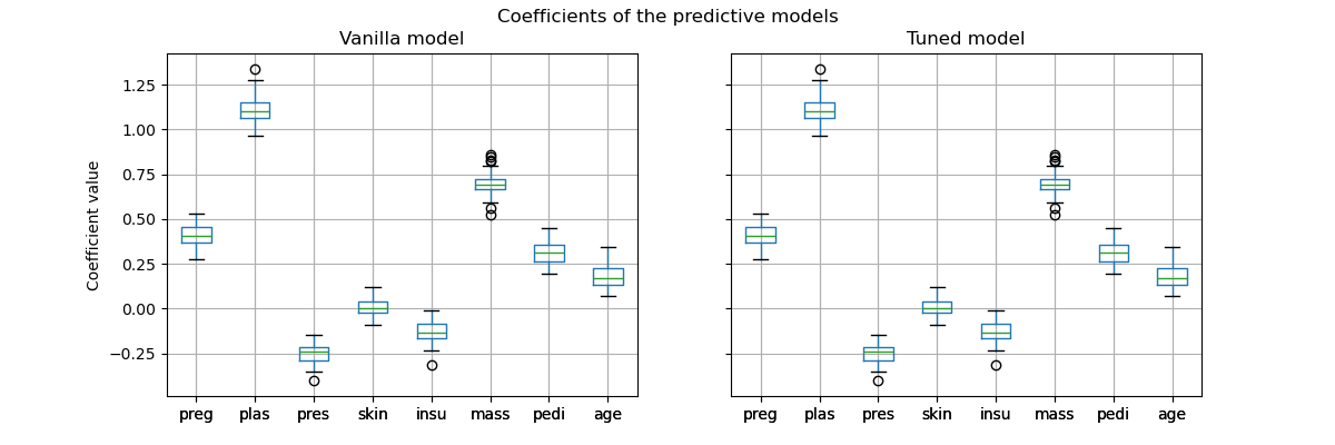
只有每个模型的决策阈值在交叉验证期间发生了改变。
decision_threshold = pd.Series(
    [est.best_threshold_ for est in cv_results_tuned_model["estimator"]],
)
ax = decision_threshold.plot.kde()
ax.axvline(
    decision_threshold.mean(),
    color="k",
    linestyle="--",
    label=f"Mean decision threshold: {decision_threshold.mean():.2f}",
)
ax.set_xlabel("Decision threshold")
ax.legend(loc="upper right")
_ = ax.set_title(
    "Distribution of the decision threshold \nacross different cross-validation folds"
)
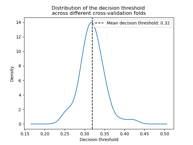
平均而言,大约 0.32 的决策阈值最大化了平衡准确率,这与默认决策阈值 0.5 不同。因此,当预测模型的输出用于做出决策时,调整决策阈值尤为重要。此外,用于调整决策阈值的度量标准应仔细选择。在这里,我们使用了平衡准确率,但这可能不是手头问题最合适的度量标准。“正确”度量标准的选择通常取决于具体问题,并且可能需要一些领域知识。有关更多详细信息,请参阅题为成本敏感学习的决策阈值事后调优的示例。
脚本总运行时间: (0 分 31.288 秒)


相关示例