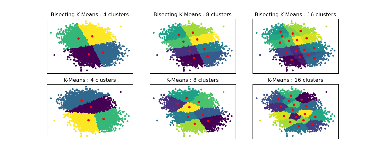
二分 K-均值与常规 K-均值性能比较#

此示例展示了常规 K-均值算法与二分 K-均值算法之间的差异。

虽然常规 K-均值聚类在增加 n_clusters 时会发生变化，但二分 K-均值聚类建立在先前的聚类之上。因此，它倾向于创建具有更规则的大尺度结构的聚类。这种差异可以通过视觉观察：对于所有聚类数量，二分 K-均值都有一条分割线将整个数据云一分为二，而常规 K-均值则没有。

Bisecting K-Means : 4 clusters, Bisecting K-Means : 8 clusters, Bisecting K-Means : 16 clusters, K-Means : 4 clusters, K-Means : 8 clusters, K-Means : 16 clusters

# Authors: The scikit-learn developers
# SPDX-License-Identifier: BSD-3-Clause

import matplotlib.pyplot as plt

from sklearn.cluster import BisectingKMeans, KMeans
from sklearn.datasets import make_blobs

# Generate sample data
n_samples = 10000
random_state = 0

X, _ = make_blobs(n_samples=n_samples, centers=2, random_state=random_state)

# Number of cluster centers for KMeans and BisectingKMeans
n_clusters_list = [4, 8, 16]

# Algorithms to compare
clustering_algorithms = {
    "Bisecting K-Means": BisectingKMeans,
    "K-Means": KMeans,
}

# Make subplots for each variant
fig, axs = plt.subplots(
    len(clustering_algorithms), len(n_clusters_list), figsize=(12, 5)
)

axs = axs.T

for i, (algorithm_name, Algorithm) in enumerate(clustering_algorithms.items()):
    for j, n_clusters in enumerate(n_clusters_list):
        algo = Algorithm(n_clusters=n_clusters, random_state=random_state, n_init=3)
        algo.fit(X)
        centers = algo.cluster_centers_

        axs[j, i].scatter(X[:, 0], X[:, 1], s=10, c=algo.labels_)
        axs[j, i].scatter(centers[:, 0], centers[:, 1], c="r", s=20)

        axs[j, i].set_title(f"{algorithm_name} : {n_clusters} clusters")


# Hide x labels and tick labels for top plots and y ticks for right plots.
for ax in axs.flat:
    ax.label_outer()
    ax.set_xticks([])
    ax.set_yticks([])

plt.show()

脚本总运行时间： (0 minutes 1.053 seconds)

二分 K-均值与常规 K-均值性能比较#

本页