使用自定义核函数的 SVM#

展示如何将支持向量机 (SVM) 分类器与自定义核函数配合使用。该示例将绘制决策曲面并突出显示支持向量。

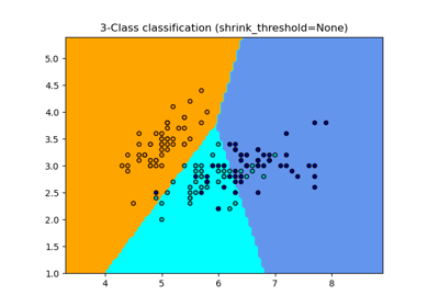
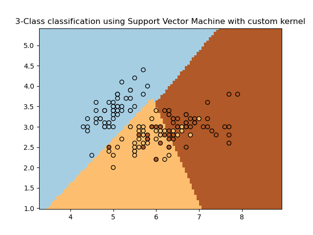
3-Class classification using Support Vector Machine with custom kernel

# Authors: The scikit-learn developers
# SPDX-License-Identifier: BSD-3-Clause

import matplotlib.pyplot as plt
import numpy as np

from sklearn import datasets, svm
from sklearn.inspection import DecisionBoundaryDisplay

# Import some data to play with.
iris = datasets.load_iris()
X = iris.data[:, :2]  # We only take the first two features. We could
# avoid this ugly slicing by using a two-dim dataset.
Y = iris.target


def my_kernel(X, Y):
    """
    We create a custom kernel:

                 (2  0)
    k(X, Y) = X  (    ) Y.T
                 (0  1)
    """
    M = np.array([[2, 0], [0, 1.0]])
    return np.dot(np.dot(X, M), Y.T)


# We create an instance of SVC with that kernel and fit it on the data.
clf = svm.SVC(kernel=my_kernel)
clf.fit(X, Y)

ax = plt.gca()
DecisionBoundaryDisplay.from_estimator(
    clf,
    X,
    multiclass_colors="Paired",
    ax=ax,
    response_method="predict",
    plot_method="pcolormesh",
    shading="auto",
    alpha=0.5,
)

# Plot the training points
plt.scatter(X[:, 0], X[:, 1], c=Y, cmap=plt.cm.Paired)
# Highlight the support vectors
plt.scatter(
    X[clf.support_, 0],
    X[clf.support_, 1],
    facecolor="none",
    edgecolors="k",
)
plt.title("3-Class classification using Support Vector Machine with custom kernel")
plt.axis("tight")
plt.show()

脚本总运行时间：（0 分 0.103 秒）