注意
跳转至末尾 下载完整示例代码。或通过 JupyterLite 或 Binder 在浏览器中运行此示例。
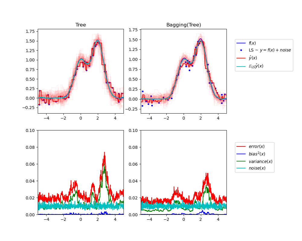
单一估计器与装袋法(Bagging):偏差-方差分解#
本示例旨在说明并比较单一估计器与装袋法(Bagging)集成模型的期望均方误差的偏差-方差分解。
在回归问题中,估计器的期望均方误差可以分解为偏差、方差和噪声。在回归问题的不同数据集上取平均值时,偏差项衡量的是估计器的预测与该问题最佳估计器(即贝叶斯模型)的预测之间的平均差异。方差项衡量的是当估计器在同一问题的不同随机实例上进行拟合时,其预测的可变性。以下将每个问题实例标记为“LS”,代表“学习样本”(Learning Sample)。最后,噪声衡量的是误差中不可约的部分,这部分误差是由数据的变异性引起的。
左上角的图展示了在玩具一维回归问题的随机数据集 LS(蓝色圆点)上训练的单一决策树的预测(深红色)。它还展示了在同一问题的其他(且不同)随机抽取的 LS 实例上训练的其他单一决策树的预测(浅红色)。直观地说,这里的方差项对应于单个估计器预测束(浅红色)的宽度。方差越大,x 的预测对训练集微小变化的敏感度就越高。偏差项对应于估计器的平均预测(青色)与最佳可能模型(深蓝色)之间的差异。在这个问题上,我们可以观察到偏差相当低(青色和蓝色曲线彼此靠近),而方差很大(红色束相当宽)。
左下角的图绘制了单一决策树期望均方误差的逐点分解。它证实了偏差项(蓝色)较低,而方差(绿色)较大。它还展示了误差中的噪声部分,正如预期,这部分噪声看起来是恒定的,大约为 0.01。
右侧的图对应相同的绘图,但改为使用决策树的装袋(bagging)集成模型。在两幅图中,我们都可以观察到偏差项比之前的情况更大。在右上图中,平均预测(青色)与最佳可能模型之间的差异更大(例如,注意 x=2 附近的偏移)。在右下图中,偏差曲线也略高于左下图中。然而,在方差方面,预测束更窄,这表明方差较低。确实,正如右下角的图所证实,方差项(绿色)低于单一决策树。因此,总体而言,偏差-方差分解不再相同。装袋法(bagging)的权衡更好:对在数据集的自助采样副本上拟合的多个决策树进行平均,会略微增加偏差项,但能更大程度地降低方差,从而降低整体均方误差(比较下方图中红色曲线)。脚本输出也证实了这一直觉。装袋集成模型的总误差低于单一决策树的总误差,这种差异确实主要源于方差的降低。
有关偏差-方差分解的更多详细信息,请参见 [1] 的第 7.3 节。
参考文献#
Tree: 0.0255 (error) = 0.0003 (bias^2)  + 0.0152 (var) + 0.0098 (noise)
Bagging(Tree): 0.0196 (error) = 0.0004 (bias^2)  + 0.0092 (var) + 0.0098 (noise)
# Authors: The scikit-learn developers
# SPDX-License-Identifier: BSD-3-Clause

import matplotlib.pyplot as plt
import numpy as np

from sklearn.ensemble import BaggingRegressor
from sklearn.tree import DecisionTreeRegressor

# Settings
n_repeat = 50  # Number of iterations for computing expectations
n_train = 50  # Size of the training set
n_test = 1000  # Size of the test set
noise = 0.1  # Standard deviation of the noise
np.random.seed(0)

# Change this for exploring the bias-variance decomposition of other
# estimators. This should work well for estimators with high variance (e.g.,
# decision trees or KNN), but poorly for estimators with low variance (e.g.,
# linear models).
estimators = [
    ("Tree", DecisionTreeRegressor()),
    ("Bagging(Tree)", BaggingRegressor(DecisionTreeRegressor())),
]

n_estimators = len(estimators)


# Generate data
def f(x):
    x = x.ravel()

    return np.exp(-(x**2)) + 1.5 * np.exp(-((x - 2) ** 2))


def generate(n_samples, noise, n_repeat=1):
    X = np.random.rand(n_samples) * 10 - 5
    X = np.sort(X)

    if n_repeat == 1:
        y = f(X) + np.random.normal(0.0, noise, n_samples)
    else:
        y = np.zeros((n_samples, n_repeat))

        for i in range(n_repeat):
            y[:, i] = f(X) + np.random.normal(0.0, noise, n_samples)

    X = X.reshape((n_samples, 1))

    return X, y


X_train = []
y_train = []

for i in range(n_repeat):
    X, y = generate(n_samples=n_train, noise=noise)
    X_train.append(X)
    y_train.append(y)

X_test, y_test = generate(n_samples=n_test, noise=noise, n_repeat=n_repeat)

plt.figure(figsize=(10, 8))

# Loop over estimators to compare
for n, (name, estimator) in enumerate(estimators):
    # Compute predictions
    y_predict = np.zeros((n_test, n_repeat))

    for i in range(n_repeat):
        estimator.fit(X_train[i], y_train[i])
        y_predict[:, i] = estimator.predict(X_test)

    # Bias^2 + Variance + Noise decomposition of the mean squared error
    y_error = np.zeros(n_test)

    for i in range(n_repeat):
        for j in range(n_repeat):
            y_error += (y_test[:, j] - y_predict[:, i]) ** 2

    y_error /= n_repeat * n_repeat

    y_noise = np.var(y_test, axis=1)
    y_bias = (f(X_test) - np.mean(y_predict, axis=1)) ** 2
    y_var = np.var(y_predict, axis=1)

    print(
        "{0}: {1:.4f} (error) = {2:.4f} (bias^2) "
        " + {3:.4f} (var) + {4:.4f} (noise)".format(
            name, np.mean(y_error), np.mean(y_bias), np.mean(y_var), np.mean(y_noise)
        )
    )

    # Plot figures
    plt.subplot(2, n_estimators, n + 1)
    plt.plot(X_test, f(X_test), "b", label="$f(x)$")
    plt.plot(X_train[0], y_train[0], ".b", label="LS ~ $y = f(x)+noise$")

    for i in range(n_repeat):
        if i == 0:
            plt.plot(X_test, y_predict[:, i], "r", label=r"$\^y(x)$")
        else:
            plt.plot(X_test, y_predict[:, i], "r", alpha=0.05)

    plt.plot(X_test, np.mean(y_predict, axis=1), "c", label=r"$\mathbb{E}_{LS} \^y(x)$")

    plt.xlim([-5, 5])
    plt.title(name)

    if n == n_estimators - 1:
        plt.legend(loc=(1.1, 0.5))

    plt.subplot(2, n_estimators, n_estimators + n + 1)
    plt.plot(X_test, y_error, "r", label="$error(x)$")
    plt.plot(X_test, y_bias, "b", label="$bias^2(x)$")
    plt.plot(X_test, y_var, "g", label="$variance(x)$")
    plt.plot(X_test, y_noise, "c", label="$noise(x)$")

    plt.xlim([-5, 5])
    plt.ylim([0, 0.1])

    if n == n_estimators - 1:
        plt.legend(loc=(1.1, 0.5))

plt.subplots_adjust(right=0.75)
plt.show()
脚本总运行时间: (0 分 1.151 秒)
相关示例