比较交叉分解方法

各种交叉分解算法的简单用法

• PLSCanonical

• PLSRegression，具有多元响应，又名 PLS2

• PLSRegression，具有单变量响应，又名 PLS1

• CCA

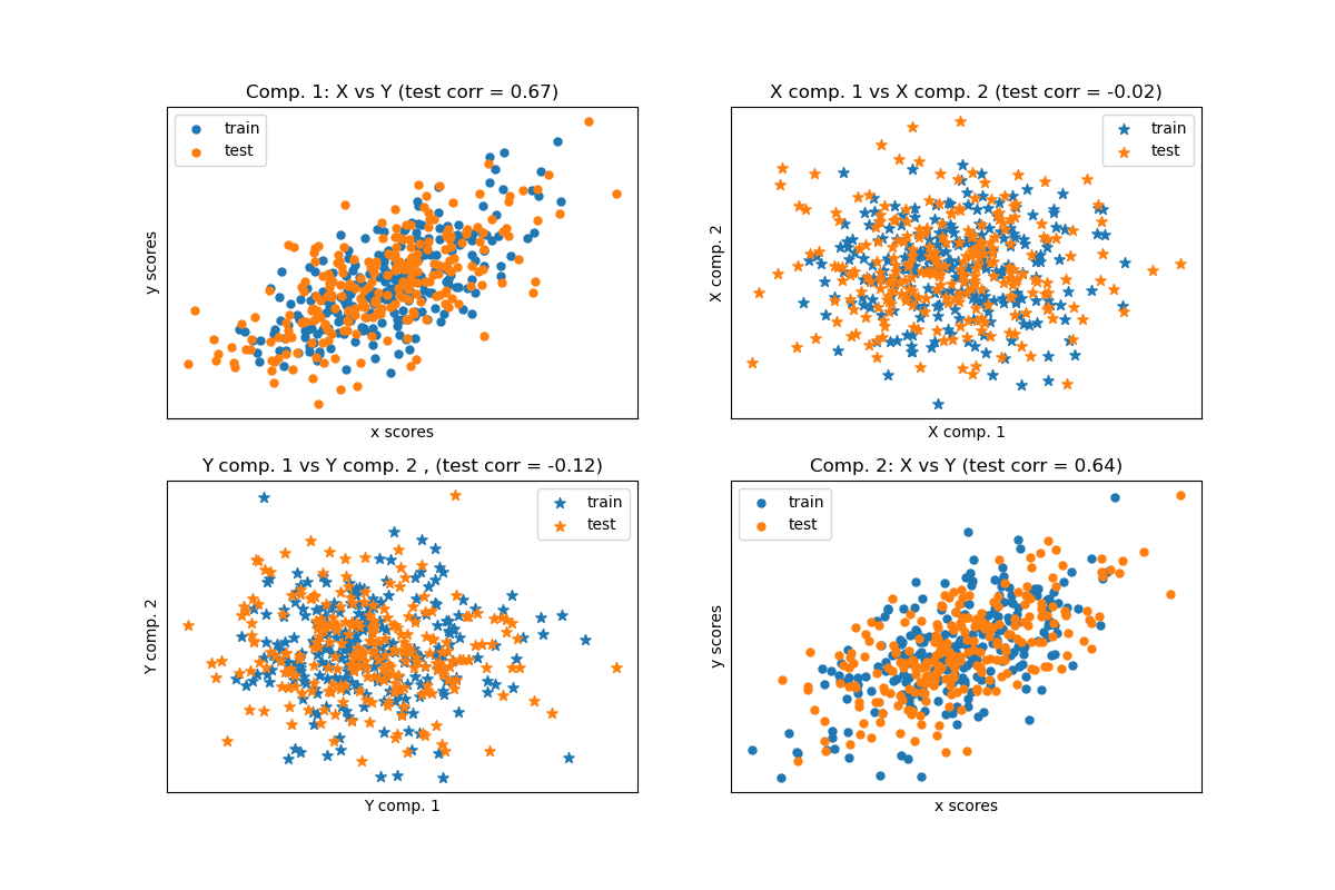
给定两个多变量协变的二维数据集 X 和 Y，PLS 提取“协方差方向”，即解释两个数据集之间最多共享方差的每个数据集的成分。这在散点图矩阵显示中很明显：数据集 X 和数据集 Y 中的成分 1 最大相关（点位于第一对角线附近）。成分 2 在两个数据集中也是如此，然而，不同成分之间跨数据集的相关性较弱：点云非常球形。

# Authors: The scikit-learn developers
# SPDX-License-Identifier: BSD-3-Clause

基于数据集的潜在变量模型

import numpy as np

from sklearn.model_selection import train_test_split

rng = np.random.default_rng(42)

n = 500
# 2 latents vars:
l1 = rng.normal(size=n)
l2 = rng.normal(size=n)

latents = np.array([l1, l1, l2, l2]).T
X = latents + rng.normal(size=(n, 4))
Y = latents + rng.normal(size=(n, 4))

X_train, X_test, Y_train, Y_test = train_test_split(X, Y, test_size=0.5, shuffle=False)

print("Corr(X)")
print(np.round(np.corrcoef(X.T), 2))
print("Corr(Y)")
print(np.round(np.corrcoef(Y.T), 2))

Corr(X)
[[ 1.    0.48 -0.01  0.  ]
 [ 0.48  1.   -0.01  0.  ]
 [-0.01 -0.01  1.    0.49]
 [ 0.    0.    0.49  1.  ]]
Corr(Y)
[[ 1.    0.47  0.03  0.05]
 [ 0.47  1.    0.03 -0.01]
 [ 0.03  0.03  1.    0.5 ]
 [ 0.05 -0.01  0.5   1.  ]]

典型（对称）PLS

转换数据

from sklearn.cross_decomposition import PLSCanonical

plsca = PLSCanonical(n_components=2)
plsca.fit(X_train, Y_train)
X_train_r, Y_train_r = plsca.transform(X_train, Y_train)
X_test_r, Y_test_r = plsca.transform(X_test, Y_test)

分数散点图

import matplotlib.pyplot as plt

# On diagonal plot X vs Y scores on each components
plt.figure(figsize=(12, 8))
plt.subplot(221)
plt.scatter(X_train_r[:, 0], Y_train_r[:, 0], label="train", marker="o", s=25)
plt.scatter(X_test_r[:, 0], Y_test_r[:, 0], label="test", marker="o", s=25)
plt.xlabel("x scores")
plt.ylabel("y scores")
plt.title(
    "Comp. 1: X vs Y (test corr = %.2f)"
    % np.corrcoef(X_test_r[:, 0], Y_test_r[:, 0])[0, 1]
)
plt.xticks(())
plt.yticks(())
plt.legend(loc="best")

plt.subplot(224)
plt.scatter(X_train_r[:, 1], Y_train_r[:, 1], label="train", marker="o", s=25)
plt.scatter(X_test_r[:, 1], Y_test_r[:, 1], label="test", marker="o", s=25)
plt.xlabel("x scores")
plt.ylabel("y scores")
plt.title(
    "Comp. 2: X vs Y (test corr = %.2f)"
    % np.corrcoef(X_test_r[:, 1], Y_test_r[:, 1])[0, 1]
)
plt.xticks(())
plt.yticks(())
plt.legend(loc="best")

# Off diagonal plot components 1 vs 2 for X and Y
plt.subplot(222)
plt.scatter(X_train_r[:, 0], X_train_r[:, 1], label="train", marker="*", s=50)
plt.scatter(X_test_r[:, 0], X_test_r[:, 1], label="test", marker="*", s=50)
plt.xlabel("X comp. 1")
plt.ylabel("X comp. 2")
plt.title(
    "X comp. 1 vs X comp. 2 (test corr = %.2f)"
    % np.corrcoef(X_test_r[:, 0], X_test_r[:, 1])[0, 1]
)
plt.legend(loc="best")
plt.xticks(())
plt.yticks(())

plt.subplot(223)
plt.scatter(Y_train_r[:, 0], Y_train_r[:, 1], label="train", marker="*", s=50)
plt.scatter(Y_test_r[:, 0], Y_test_r[:, 1], label="test", marker="*", s=50)
plt.xlabel("Y comp. 1")
plt.ylabel("Y comp. 2")
plt.title(
    "Y comp. 1 vs Y comp. 2 , (test corr = %.2f)"
    % np.corrcoef(Y_test_r[:, 0], Y_test_r[:, 1])[0, 1]
)
plt.legend(loc="best")
plt.xticks(())
plt.yticks(())
plt.show()

PLS 回归，具有多元响应，又名 PLS2

from sklearn.cross_decomposition import PLSRegression

n = 1000
q = 3
p = 10
X = rng.normal(size=(n, p))
B = np.array([[1, 2] + [0] * (p - 2)] * q).T
# each Yj = 1*X1 + 2*X2 + noize
Y = np.dot(X, B) + rng.normal(size=(n, q)) + 5

pls2 = PLSRegression(n_components=3)
pls2.fit(X, Y)
print("True B (such that: Y = XB + Err)")
print(B)
# compare pls2.coef_ with B
print("Estimated B")
print(np.round(pls2.coef_, 1))
pls2.predict(X)

True B (such that: Y = XB + Err)
[[1 1 1]
 [2 2 2]
 [0 0 0]
 [0 0 0]
 [0 0 0]
 [0 0 0]
 [0 0 0]
 [0 0 0]
 [0 0 0]
 [0 0 0]]
Estimated B
[[ 1.   2.   0.  -0.   0.   0.   0.   0.   0.  -0. ]
 [ 1.   2.   0.  -0.  -0.  -0.  -0.  -0.1 -0.   0. ]
 [ 1.   2.   0.  -0.   0.   0.  -0.  -0.   0.   0. ]]

array([[4.09928294, 4.27252412, 4.116446  ],
       [3.22383315, 3.36186659, 3.2829478 ],
       [6.40665836, 6.45699286, 6.28414926],
       ...,
       [1.50716084, 1.50460976, 1.5177967 ],
       [6.67188307, 6.51139993, 6.47838503],
       [5.93803911, 5.99272896, 5.91191611]], shape=(1000, 3))

PLS 回归，具有单变量响应，又名 PLS1

n = 1000
p = 10
X = rng.normal(size=(n, p))
y = X[:, 0] + 2 * X[:, 1] + rng.normal(size=n) + 5
pls1 = PLSRegression(n_components=3)
pls1.fit(X, y)
# note that the number of components exceeds 1 (the dimension of y)
print("Estimated betas")
print(np.round(pls1.coef_, 1))

Estimated betas
[[ 1.   2.  -0.   0.  -0.   0.  -0.1  0.  -0.  -0. ]]

CCA（带对称缩减的 PLS 模式 B）

from sklearn.cross_decomposition import CCA

cca = CCA(n_components=2)
cca.fit(X_train, Y_train)
X_train_r, Y_train_r = cca.transform(X_train, Y_train)
X_test_r, Y_test_r = cca.transform(X_test, Y_test)

相关示例

多标签分类

多标签分类

主成分回归 vs 偏最小二乘回归

主成分回归 vs 偏最小二乘回归

两类 AdaBoost

两类 AdaBoost

具有多重共线或相关特征的排列重要性

具有多重共线或相关特征的排列重要性