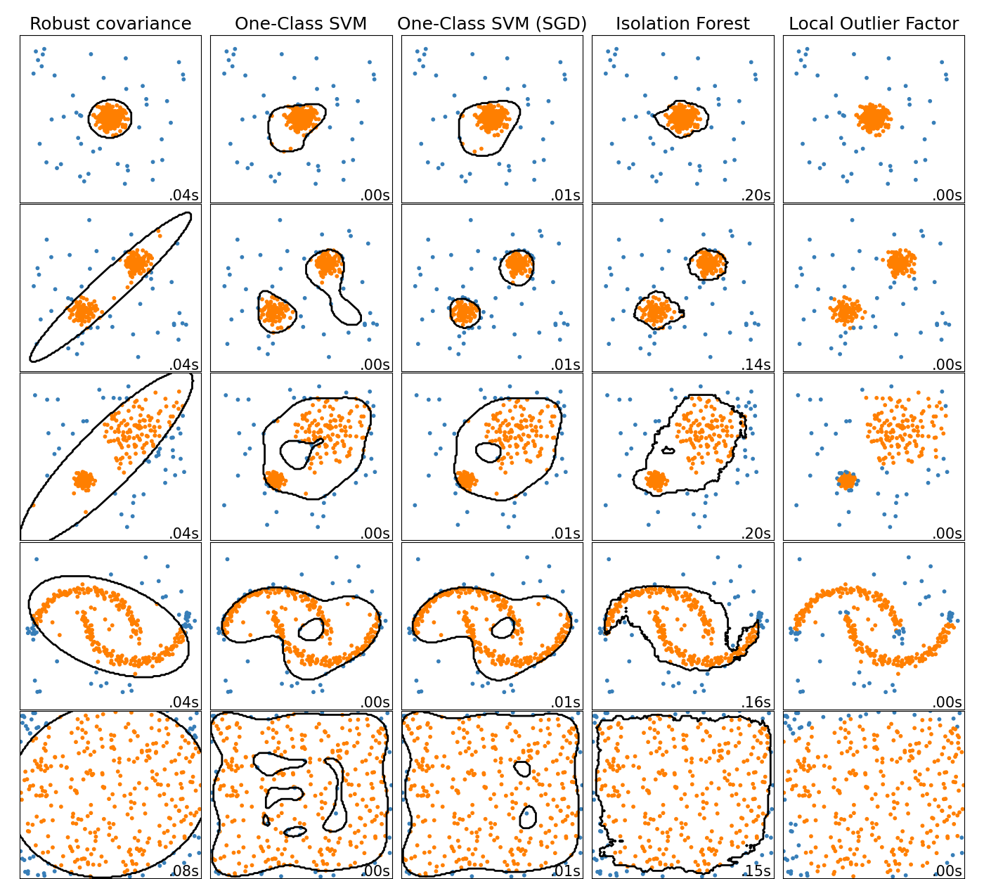
比较用于玩具数据集上离群值检测的异常检测算法#

此示例展示了不同异常检测算法在 2D 数据集上的特性。数据集包含一个或两个模式（高密度区域），以说明算法处理多模态数据的能力。

对于每个数据集，15% 的样本生成为随机均匀噪声。这个比例是赋给 OneClassSVM 的 nu 参数和其他离群值检测算法的 contamination 参数的值。内点和离群值之间的决策边界以黑色显示，除了 Local Outlier Factor (LOF)，因为它在用于离群值检测时没有可应用于新数据的 predict 方法。

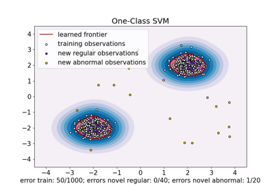
OneClassSVM 众所周知对离群值敏感，因此在离群值检测方面表现不佳。当训练集未被离群值污染时，此估计器最适合用于新颖性检测。尽管如此，在高维或对内点数据的分布没有任何假设的情况下进行离群值检测非常具有挑战性，在这种情况下，One-class SVM 可能会根据其超参数的值给出有用的结果。

sklearn.linear_model.SGDOneClassSVM 是基于随机梯度下降 (SGD) 实现的 One-Class SVM。结合核近似，此估计器可用于近似核化 sklearn.svm.OneClassSVM 的解。我们注意到，尽管不完全相同，sklearn.linear_model.SGDOneClassSVM 的决策边界与 sklearn.svm.OneClassSVM 的决策边界非常相似。使用 sklearn.linear_model.SGDOneClassSVM 的主要优点是它随样本数量线性扩展。

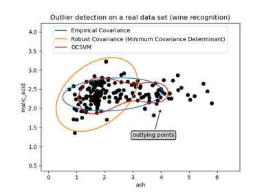
sklearn.covariance.EllipticEnvelope 假设数据是高斯分布的并学习一个椭圆。因此，当数据不是单模态时，它会退化。然而请注意，此估计器对离群值具有鲁棒性。

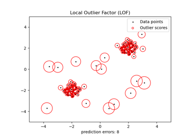
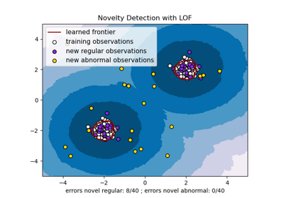
IsolationForest 和 LocalOutlierFactor 似乎在多模态数据集上表现良好。LOF 优于其他估计器的地方体现在第三个数据集上，其中两个模式具有不同的密度。这种优势通过 LOF 的局部特性来解释，这意味着它只将一个样本的异常分数与其邻居的分数进行比较。

最后，对于最后一个数据集，很难说一个样本比另一个样本更异常，因为它们均匀分布在一个超立方体中。除了 OneClassSVM 有点过拟合之外，所有估计器都为这种情况提供了体面的解决方案。在这种情况下，仔细查看样本的异常分数是明智的，因为一个好的估计器应该为所有样本分配相似的分数。

虽然这些示例提供了一些关于算法的直觉，但这种直觉可能不适用于非常高维度的数据。

最后，请注意，模型的参数在此处是手动选择的，但在实践中需要进行调整。在缺乏标记数据的情况下，问题完全是无监督的，因此模型选择可能是一个挑战。

Robust covariance, One-Class SVM, One-Class SVM (SGD), Isolation Forest, Local Outlier Factor

# Authors: The scikit-learn developers
# SPDX-License-Identifier: BSD-3-Clause

import time

import matplotlib
import matplotlib.pyplot as plt
import numpy as np

from sklearn import svm
from sklearn.covariance import EllipticEnvelope
from sklearn.datasets import make_blobs, make_moons
from sklearn.ensemble import IsolationForest
from sklearn.kernel_approximation import Nystroem
from sklearn.linear_model import SGDOneClassSVM
from sklearn.neighbors import LocalOutlierFactor
from sklearn.pipeline import make_pipeline

matplotlib.rcParams["contour.negative_linestyle"] = "solid"

# Example settings
n_samples = 300
outliers_fraction = 0.15
n_outliers = int(outliers_fraction * n_samples)
n_inliers = n_samples - n_outliers

# define outlier/anomaly detection methods to be compared.
# the SGDOneClassSVM must be used in a pipeline with a kernel approximation
# to give similar results to the OneClassSVM
anomaly_algorithms = [
    (
        "Robust covariance",
        EllipticEnvelope(contamination=outliers_fraction, random_state=42),
    ),
    ("One-Class SVM", svm.OneClassSVM(nu=outliers_fraction, kernel="rbf", gamma=0.1)),
    (
        "One-Class SVM (SGD)",
        make_pipeline(
            Nystroem(gamma=0.1, random_state=42, n_components=150),
            SGDOneClassSVM(
                nu=outliers_fraction,
                shuffle=True,
                fit_intercept=True,
                random_state=42,
                tol=1e-6,
            ),
        ),
    ),
    (
        "Isolation Forest",
        IsolationForest(contamination=outliers_fraction, random_state=42),
    ),
    (
        "Local Outlier Factor",
        LocalOutlierFactor(n_neighbors=35, contamination=outliers_fraction),
    ),
]

# Define datasets
blobs_params = dict(random_state=0, n_samples=n_inliers, n_features=2)
datasets = [
    make_blobs(centers=[[0, 0], [0, 0]], cluster_std=0.5, **blobs_params)[0],
    make_blobs(centers=[[2, 2], [-2, -2]], cluster_std=[0.5, 0.5], **blobs_params)[0],
    make_blobs(centers=[[2, 2], [-2, -2]], cluster_std=[1.5, 0.3], **blobs_params)[0],
    4.0
    * (
        make_moons(n_samples=n_samples, noise=0.05, random_state=0)[0]
        - np.array([0.5, 0.25])
    ),
    14.0 * (np.random.RandomState(42).rand(n_samples, 2) - 0.5),
]

# Compare given classifiers under given settings
xx, yy = np.meshgrid(np.linspace(-7, 7, 150), np.linspace(-7, 7, 150))

plt.figure(figsize=(len(anomaly_algorithms) * 2 + 4, 12.5))
plt.subplots_adjust(
    left=0.02, right=0.98, bottom=0.001, top=0.96, wspace=0.05, hspace=0.01
)

plot_num = 1
rng = np.random.RandomState(42)

for i_dataset, X in enumerate(datasets):
    # Add outliers
    X = np.concatenate([X, rng.uniform(low=-6, high=6, size=(n_outliers, 2))], axis=0)

    for name, algorithm in anomaly_algorithms:
        t0 = time.time()
        algorithm.fit(X)
        t1 = time.time()
        plt.subplot(len(datasets), len(anomaly_algorithms), plot_num)
        if i_dataset == 0:
            plt.title(name, size=18)

        # fit the data and tag outliers
        if name == "Local Outlier Factor":
            y_pred = algorithm.fit_predict(X)
        else:
            y_pred = algorithm.fit(X).predict(X)

        # plot the levels lines and the points
        if name != "Local Outlier Factor":  # LOF does not implement predict
            Z = algorithm.predict(np.c_[xx.ravel(), yy.ravel()])
            Z = Z.reshape(xx.shape)
            plt.contour(xx, yy, Z, levels=[0], linewidths=2, colors="black")

        colors = np.array(["#377eb8", "#ff7f00"])
        plt.scatter(X[:, 0], X[:, 1], s=10, color=colors[(y_pred + 1) // 2])

        plt.xlim(-7, 7)
        plt.ylim(-7, 7)
        plt.xticks(())
        plt.yticks(())
        plt.text(
            0.99,
            0.01,
            ("%.2fs" % (t1 - t0)).lstrip("0"),
            transform=plt.gca().transAxes,
            size=15,
            horizontalalignment="right",
        )
        plot_num += 1

plt.show()

脚本总运行时间： (0 分钟 3.269 秒)

比较用于玩具数据集上离群值检测的异常检测算法#

本页