注意
转到末尾以下载完整示例代码,或通过 JupyterLite 或 Binder 在浏览器中运行此示例。
时间相关特征工程#
本笔记本介绍了利用时间相关特征进行共享单车需求回归任务的不同策略,该任务高度依赖于业务周期(天、周、月)和年度季节周期。
在此过程中,我们介绍了如何使用 sklearn.preprocessing.SplineTransformer 类及其 extrapolation="periodic" 选项执行周期性特征工程。
# Authors: The scikit-learn developers
# SPDX-License-Identifier: BSD-3-Clause
共享单车需求数据集上的数据探索#
我们首先从 OpenML 仓库加载数据。
from sklearn.datasets import fetch_openml

bike_sharing = fetch_openml("Bike_Sharing_Demand", version=2, as_frame=True)
df = bike_sharing.frame
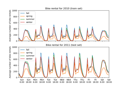
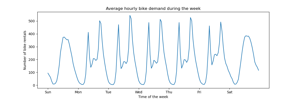
为了快速了解数据的周期性模式,我们来看看一周内每小时的平均需求。
请注意,一周从周日开始,正值周末。我们可以清楚地分辨工作日早晚高峰的通勤模式,以及周末自行车更广泛的休闲使用模式,其高峰需求集中在白天中部。
import matplotlib.pyplot as plt

fig, ax = plt.subplots(figsize=(12, 4))
average_week_demand = df.groupby(["weekday", "hour"])["count"].mean()
average_week_demand.plot(ax=ax)
_ = ax.set(
    title="Average hourly bike demand during the week",
    xticks=[i * 24 for i in range(7)],
    xticklabels=["Sun", "Mon", "Tue", "Wed", "Thu", "Fri", "Sat"],
    xlabel="Time of the week",
    ylabel="Number of bike rentals",
)
预测问题的目标是每小时自行车租赁的绝对数量。
df["count"].max()
np.int64(977)
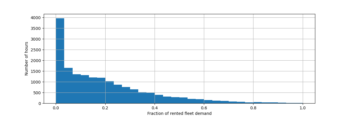
让我们重新缩放目标变量(每小时自行车租赁数量),以预测相对需求,这样平均绝对误差更容易被解释为最大需求的一个分数。
注意
本笔记本中使用的模型的拟合方法都通过最小化均方误差来估计条件均值。然而,绝对误差会估计条件中位数。
尽管如此,在讨论中报告测试集上的性能度量时,我们选择侧重于平均绝对误差而不是(根)均方误差,因为它更直观易懂。然而请注意,在本研究中,一个度量的最佳模型在另一个度量方面也是最佳的。
y = df["count"] / df["count"].max()
fig, ax = plt.subplots(figsize=(12, 4))
y.hist(bins=30, ax=ax)
_ = ax.set(
    xlabel="Fraction of rented fleet demand",
    ylabel="Number of hours",
)
输入特征数据帧是描述天气状况的带时间注释的每小时变量日志。它包括数值变量和分类变量。请注意,时间信息已扩展为几个互补的列。
X = df.drop("count", axis="columns")
X
注意
如果时间信息仅以日期或日期时间列的形式存在,我们可以使用 pandas 将其扩展为日内小时、周内天数、月内天数、年内月份:https://pandas.ac.cn/pandas-docs/stable/user_guide/timeseries.html#time-date-components
现在我们检查分类变量的分布,从 "weather" 开始。
X["weather"].value_counts()
weather
clear         11413
misty          4544
rain           1419
heavy_rain        3
Name: count, dtype: int64
由于只有 3 个 "heavy_rain" 事件,我们不能使用此类别进行交叉验证的机器学习模型训练。相反,我们通过将其合并到 "rain" 类别来简化表示。
X["weather"] = (
    X["weather"]
    .astype(object)
    .replace(to_replace="heavy_rain", value="rain")
    .astype("category")
)
X["weather"].value_counts()
weather
clear    11413
misty     4544
rain      1422
Name: count, dtype: int64
正如所料,"season" 变量分布均衡。
X["season"].value_counts()
season
fall      4496
summer    4409
spring    4242
winter    4232
Name: count, dtype: int64
基于时间的交叉验证#
由于数据集是时间有序的事件日志(每小时需求),我们将使用时间敏感的交叉验证分割器来尽可能真实地评估我们的需求预测模型。我们在分割的训练集和测试集之间使用了 2 天的间隔。我们还限制了训练集的大小,以使交叉验证折叠的性能更稳定。
1000 个测试数据点应该足以量化模型的性能。这相当于不到一个半月的连续测试数据。
from sklearn.model_selection import TimeSeriesSplit

ts_cv = TimeSeriesSplit(
    n_splits=5,
    gap=48,
    max_train_size=10000,
    test_size=1000,
)
让我们手动检查各个分割,以确认 TimeSeriesSplit 按预期工作,从第一个分割开始。
all_splits = list(ts_cv.split(X, y))
train_0, test_0 = all_splits[0]
X.iloc[test_0]
X.iloc[train_0]
现在我们检查最后一个分割。
train_4, test_4 = all_splits[4]
X.iloc[test_4]
X.iloc[train_4]
一切顺利。现在我们准备进行一些预测建模!
梯度提升#
结合决策树的梯度提升回归通常足够灵活,只要样本数量足够大,就能有效处理混合了分类和数值特征的异构表格数据。
在这里,我们使用现代的 HistGradientBoostingRegressor,它本地支持分类特征。因此,我们只需设置 categorical_features="from_dtype",以便具有分类数据类型的特征被视为分类特征。作为参考,我们根据数据类型从数据帧中提取分类特征。内部树对这些特征使用专门的树分割规则。
数值变量无需预处理,为简单起见,我们仅尝试此模型的默认超参数。
from sklearn.compose import ColumnTransformer
from sklearn.ensemble import HistGradientBoostingRegressor
from sklearn.model_selection import cross_validate
from sklearn.pipeline import make_pipeline

gbrt = HistGradientBoostingRegressor(categorical_features="from_dtype", random_state=42)
categorical_columns = X.columns[X.dtypes == "category"]
print("Categorical features:", categorical_columns.tolist())
Categorical features: ['season', 'holiday', 'workingday', 'weather']
让我们使用相对需求的平均绝对误差来评估我们的梯度提升模型,该误差通过我们 5 个基于时间的交叉验证分割进行平均。
import numpy as np


def evaluate(model, X, y, cv, model_prop=None, model_step=None):
    cv_results = cross_validate(
        model,
        X,
        y,
        cv=cv,
        scoring=["neg_mean_absolute_error", "neg_root_mean_squared_error"],
        return_estimator=model_prop is not None,
    )
    if model_prop is not None:
        if model_step is not None:
            values = [
                getattr(m[model_step], model_prop) for m in cv_results["estimator"]
            ]
        else:
            values = [getattr(m, model_prop) for m in cv_results["estimator"]]
        print(f"Mean model.{model_prop} = {np.mean(values)}")
    mae = -cv_results["test_neg_mean_absolute_error"]
    rmse = -cv_results["test_neg_root_mean_squared_error"]
    print(
        f"Mean Absolute Error:     {mae.mean():.3f} +/- {mae.std():.3f}\n"
        f"Root Mean Squared Error: {rmse.mean():.3f} +/- {rmse.std():.3f}"
    )


evaluate(gbrt, X, y, cv=ts_cv, model_prop="n_iter_")
Mean model.n_iter_ = 100.0
Mean Absolute Error:     0.044 +/- 0.003
Root Mean Squared Error: 0.068 +/- 0.005
我们看到我们将 max_iter 设置得足够大,以便触发了早期停止。
该模型的平均误差约为最大需求的 4% 到 5%。对于没有进行任何超参数调优的首次尝试来说,这相当不错!我们只需明确分类变量。请注意,时间相关特征是按原样传递的,即未经过处理。但这对于基于树的模型来说问题不大,因为它们可以学习有序输入特征与目标之间的非单调关系。
但对于线性回归模型来说并非如此,我们将在下文中看到。
朴素线性回归#
与线性模型通常一样,分类变量需要进行独热编码。为保持一致性,我们使用 MinMaxScaler 将数值特征缩放到相同的 0-1 范围,尽管在此例中它对结果影响不大,因为它们已经处于可比较的尺度。
from sklearn.linear_model import RidgeCV
from sklearn.preprocessing import MinMaxScaler, OneHotEncoder

one_hot_encoder = OneHotEncoder(handle_unknown="ignore", sparse_output=False)
alphas = np.logspace(-6, 6, 25)
naive_linear_pipeline = make_pipeline(
    ColumnTransformer(
        transformers=[
            ("categorical", one_hot_encoder, categorical_columns),
        ],
        remainder=MinMaxScaler(),
    ),
    RidgeCV(alphas=alphas),
)


evaluate(
    naive_linear_pipeline, X, y, cv=ts_cv, model_prop="alpha_", model_step="ridgecv"
)
Mean model.alpha_ = 2.7298221281347037
Mean Absolute Error:     0.142 +/- 0.014
Root Mean Squared Error: 0.184 +/- 0.020
确认选定的 alpha_ 在我们指定的范围内。
性能不佳:平均误差约为最大需求的 14%。这比梯度提升模型的平均误差高出三倍多。我们可以怀疑,周期性时间相关特征的朴素原始编码(仅进行最小-最大缩放)可能阻止了线性回归模型充分利用时间信息:线性回归不会自动建模输入特征与目标之间的非单调关系。非线性项必须在输入中进行特征工程。
例如,"hour" 特征的原始数值编码使得线性模型无法识别:早上 6 点到 8 点小时数的增加应该对自行车租赁数量产生强烈的正向影响,而晚上 18 点到 20 点类似幅度的增加应该对预测的自行车租赁数量产生强烈的负向影响。
将时间步长视为类别#
由于时间特征以离散方式使用整数编码(“小时”特征中有 24 个唯一值),我们可以决定使用独热编码将这些特征视为分类变量,从而忽略小时值排序所隐含的任何假设。
对时间特征使用独热编码为线性模型提供了更大的灵活性,因为我们为每个离散时间级别引入了一个额外的特征。
one_hot_linear_pipeline = make_pipeline(
    ColumnTransformer(
        transformers=[
            ("categorical", one_hot_encoder, categorical_columns),
            ("one_hot_time", one_hot_encoder, ["hour", "weekday", "month"]),
        ],
        remainder=MinMaxScaler(),
    ),
    RidgeCV(alphas=alphas),
)

evaluate(one_hot_linear_pipeline, X, y, cv=ts_cv)
Mean Absolute Error:     0.099 +/- 0.011
Root Mean Squared Error: 0.131 +/- 0.011
该模型的平均错误率是 10%,这比使用时间特征的原始(有序)编码要好得多,证实了我们的直觉:线性回归模型受益于不以单调方式处理时间进程所带来的额外灵活性。
然而,这引入了大量的新的特征。如果一天中的时间表示为自一天开始以来的分钟数而不是小时数,独热编码将引入 1440 个特征而不是 24 个。这可能会导致显著的过拟合。为了避免这种情况,我们可以使用 sklearn.preprocessing.KBinsDiscretizer 来重新分箱细粒度有序或数值变量的级别数量,同时仍然受益于独热编码的非单调表达优势。
最后,我们还观察到独热编码完全忽略了小时级别的排序,而这可能是一个值得在一定程度上保留的有趣归纳偏置。在下文中,我们将尝试探索平滑的、非单调的编码,它在局部保留时间特征的相对顺序。
三角函数特征#
作为第一次尝试,我们可以尝试使用匹配周期的正弦和余弦变换来编码这些周期性特征。
每个有序时间特征都被转换成 2 个特征,它们共同以非单调的方式编码等价信息,更重要的是,在周期范围的第一个值和最后一个值之间没有任何跳跃。
from sklearn.preprocessing import FunctionTransformer


def sin_transformer(period):
    return FunctionTransformer(lambda x: np.sin(x / period * 2 * np.pi))


def cos_transformer(period):
    return FunctionTransformer(lambda x: np.cos(x / period * 2 * np.pi))
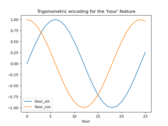
让我们可视化这种特征扩展对一些合成小时数据的影响,其中包含一些超出 23 小时的外推。
import pandas as pd

hour_df = pd.DataFrame(
    np.arange(26).reshape(-1, 1),
    columns=["hour"],
)
hour_df["hour_sin"] = sin_transformer(24).fit_transform(hour_df)["hour"]
hour_df["hour_cos"] = cos_transformer(24).fit_transform(hour_df)["hour"]
hour_df.plot(x="hour")
_ = plt.title("Trigonometric encoding for the 'hour' feature")
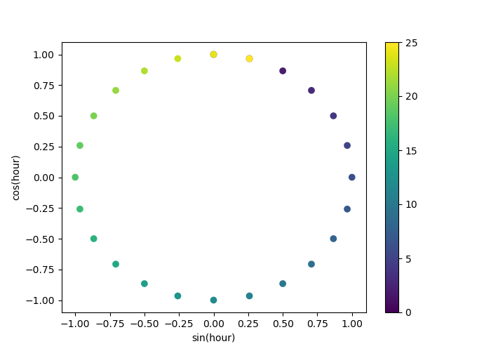
让我们使用一个 2D 散点图,其中小时数以颜色编码,以便更好地了解这种表示如何将一天中的 24 小时映射到 2D 空间,类似于某种 24 小时版本的模拟时钟。请注意,由于正弦/余弦表示的周期性,第“25”小时被映射回第 1 小时。
fig, ax = plt.subplots(figsize=(7, 5))
sp = ax.scatter(hour_df["hour_sin"], hour_df["hour_cos"], c=hour_df["hour"])
ax.set(
    xlabel="sin(hour)",
    ylabel="cos(hour)",
)
_ = fig.colorbar(sp)
现在我们可以使用这种策略构建一个特征提取流水线。
cyclic_cossin_transformer = ColumnTransformer(
    transformers=[
        ("categorical", one_hot_encoder, categorical_columns),
        ("month_sin", sin_transformer(12), ["month"]),
        ("month_cos", cos_transformer(12), ["month"]),
        ("weekday_sin", sin_transformer(7), ["weekday"]),
        ("weekday_cos", cos_transformer(7), ["weekday"]),
        ("hour_sin", sin_transformer(24), ["hour"]),
        ("hour_cos", cos_transformer(24), ["hour"]),
    ],
    remainder=MinMaxScaler(),
)
cyclic_cossin_linear_pipeline = make_pipeline(
    cyclic_cossin_transformer,
    RidgeCV(alphas=alphas),
)
evaluate(cyclic_cossin_linear_pipeline, X, y, cv=ts_cv)
Mean Absolute Error:     0.125 +/- 0.014
Root Mean Squared Error: 0.166 +/- 0.020
我们的线性回归模型在经过这种简单特征工程后的性能比使用原始有序时间特征略好,但比使用独热编码时间特征差。我们将在本笔记本末尾进一步分析导致这一令人失望结果的可能原因。
周期样条特征#
我们可以尝试使用样条变换来替代编码周期性时间相关特征,其中样条数量足够大,因此与正弦/余弦变换相比,生成的扩展特征数量也更大。
from sklearn.preprocessing import SplineTransformer


def periodic_spline_transformer(period, n_splines=None, degree=3):
    if n_splines is None:
        n_splines = period
    n_knots = n_splines + 1  # periodic and include_bias is True
    return SplineTransformer(
        degree=degree,
        n_knots=n_knots,
        knots=np.linspace(0, period, n_knots).reshape(n_knots, 1),
        extrapolation="periodic",
        include_bias=True,
    )
同样,让我们可视化这种特征扩展对一些合成小时数据的影响,其中包含一些超出 23 小时的外推。
hour_df = pd.DataFrame(
    np.linspace(0, 26, 1000).reshape(-1, 1),
    columns=["hour"],
)
splines = periodic_spline_transformer(24, n_splines=12).fit_transform(hour_df)
splines_df = pd.DataFrame(
    splines,
    columns=[f"spline_{i}" for i in range(splines.shape[1])],
)
pd.concat([hour_df, splines_df], axis="columns").plot(x="hour", cmap=plt.cm.tab20b)
_ = plt.title("Periodic spline-based encoding for the 'hour' feature")
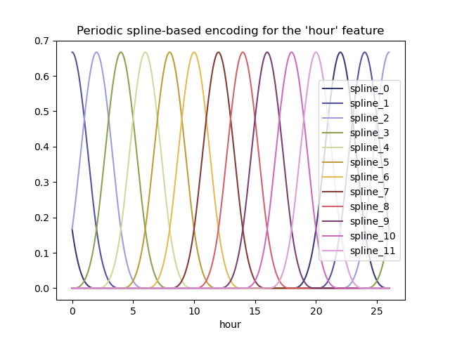
由于使用了 extrapolation="periodic" 参数,我们观察到特征编码在午夜后外推时保持平滑。
现在我们可以使用这种替代的周期性特征工程策略构建一个预测流水线。
对于这些有序值,可以使用比离散级别更少的样条。这使得基于样条的编码比独热编码更高效,同时保留了大部分表达能力。
cyclic_spline_transformer = ColumnTransformer(
    transformers=[
        ("categorical", one_hot_encoder, categorical_columns),
        ("cyclic_month", periodic_spline_transformer(12, n_splines=6), ["month"]),
        ("cyclic_weekday", periodic_spline_transformer(7, n_splines=3), ["weekday"]),
        ("cyclic_hour", periodic_spline_transformer(24, n_splines=12), ["hour"]),
    ],
    remainder=MinMaxScaler(),
)
cyclic_spline_linear_pipeline = make_pipeline(
    cyclic_spline_transformer,
    RidgeCV(alphas=alphas),
)
evaluate(cyclic_spline_linear_pipeline, X, y, cv=ts_cv)
Mean Absolute Error:     0.097 +/- 0.011
Root Mean Squared Error: 0.132 +/- 0.013
样条特征使得线性模型能够成功利用周期性时间相关特征,并将误差从最大需求的约 14% 降低到约 10%,这与我们使用独热编码特征观察到的结果相似。
特征对线性模型预测影响的定性分析#
在这里,我们希望可视化特征工程选择对预测时间相关形状的影响。
为此,我们考虑一个任意的基于时间的分割,以比较在一系列留出数据点上的预测。
naive_linear_pipeline.fit(X.iloc[train_0], y.iloc[train_0])
naive_linear_predictions = naive_linear_pipeline.predict(X.iloc[test_0])

one_hot_linear_pipeline.fit(X.iloc[train_0], y.iloc[train_0])
one_hot_linear_predictions = one_hot_linear_pipeline.predict(X.iloc[test_0])

cyclic_cossin_linear_pipeline.fit(X.iloc[train_0], y.iloc[train_0])
cyclic_cossin_linear_predictions = cyclic_cossin_linear_pipeline.predict(X.iloc[test_0])

cyclic_spline_linear_pipeline.fit(X.iloc[train_0], y.iloc[train_0])
cyclic_spline_linear_predictions = cyclic_spline_linear_pipeline.predict(X.iloc[test_0])
我们通过放大测试集的最后 96 小时(4 天)来可视化这些预测,以获得一些定性洞察。
last_hours = slice(-96, None)
fig, ax = plt.subplots(figsize=(12, 4))
fig.suptitle("Predictions by linear models")
ax.plot(
    y.iloc[test_0].values[last_hours],
    "x-",
    alpha=0.2,
    label="Actual demand",
    color="black",
)
ax.plot(naive_linear_predictions[last_hours], "x-", label="Ordinal time features")
ax.plot(
    cyclic_cossin_linear_predictions[last_hours],
    "x-",
    label="Trigonometric time features",
)
ax.plot(
    cyclic_spline_linear_predictions[last_hours],
    "x-",
    label="Spline-based time features",
)
ax.plot(
    one_hot_linear_predictions[last_hours],
    "x-",
    label="One-hot time features",
)
_ = ax.legend()
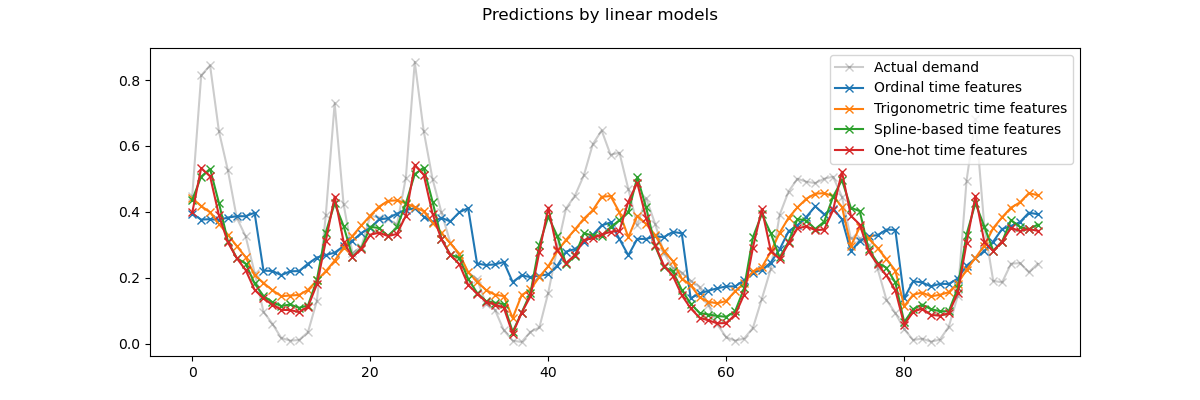
我们可以从上图中得出以下结论
原始有序时间相关特征存在问题,因为它们没有捕获自然周期性:我们观察到每天结束时,当小时特征从 23 回到 0 时,预测值会出现大幅跳跃。我们可以预期在每周或每年结束时也会出现类似的伪影。
正如所料,三角函数特征(正弦和余弦)在午夜时没有这些不连续性,但线性回归模型未能利用这些特征来正确建模日内变化。为高次谐波使用三角函数特征,或为自然周期使用具有不同相位的额外三角函数特征,可能会解决这个问题。
周期样条特征同时解决了这两个问题:通过使用 12 个样条,它们使线性模型能够聚焦于特定小时,从而赋予模型更大的表达能力。此外,
extrapolation="periodic"选项强制在hour=23和hour=0之间实现平滑表示。独热编码特征的行为与周期样条特征相似,但更具尖锐性:例如,它们可以更好地模拟工作日早晨高峰,因为这个高峰持续时间不到一小时。然而,我们将在下文看到,对于线性模型来说的优势,对于表达能力更强的模型来说不一定如此。
我们还可以比较每个特征工程流水线提取的特征数量。
naive_linear_pipeline[:-1].transform(X).shape
(17379, 19)
one_hot_linear_pipeline[:-1].transform(X).shape
(17379, 59)
cyclic_cossin_linear_pipeline[:-1].transform(X).shape
(17379, 22)
cyclic_spline_linear_pipeline[:-1].transform(X).shape
(17379, 37)
这证实了独热编码和样条编码策略为时间表示创建了比替代方案更多的特征,这反过来又为下游线性模型提供了更大的灵活性(自由度),以避免欠拟合。
最后,我们观察到所有线性模型都无法近似真实的自行车租赁需求,特别是对于工作日高峰期非常尖锐而周末平坦得多的峰值:基于样条或独热编码的最精确线性模型倾向于即使在周末也预测与通勤相关的自行车租赁高峰,并低估工作日期间与通勤相关的事件。
这些系统性预测误差揭示了一种欠拟合形式,可以通过特征之间缺乏交互项来解释,例如“workingday”和从“hours”派生出的特征。这个问题将在下一节中解决。
使用样条和多项式特征建模成对交互#
线性模型不会自动捕获输入特征之间的交互效应。一些特征是边际非线性的,例如由 SplineTransformer(或独热编码或分箱)构建的特征,这无济于事。
然而,可以使用 PolynomialFeatures 类对粗粒度样条编码小时进行处理,以显式建模“workingday”/“hours”交互,而不会引入过多新变量。
from sklearn.pipeline import FeatureUnion
from sklearn.preprocessing import PolynomialFeatures

hour_workday_interaction = make_pipeline(
    ColumnTransformer(
        [
            ("cyclic_hour", periodic_spline_transformer(24, n_splines=8), ["hour"]),
            ("workingday", FunctionTransformer(lambda x: x == "True"), ["workingday"]),
        ]
    ),
    PolynomialFeatures(degree=2, interaction_only=True, include_bias=False),
)
这些特征随后与先前基于样条的流水线中已计算的特征相结合。通过显式建模这种成对交互,我们可以观察到显著的性能改进。
cyclic_spline_interactions_pipeline = make_pipeline(
    FeatureUnion(
        [
            ("marginal", cyclic_spline_transformer),
            ("interactions", hour_workday_interaction),
        ]
    ),
    RidgeCV(alphas=alphas),
)
evaluate(cyclic_spline_interactions_pipeline, X, y, cv=ts_cv)
Mean Absolute Error:     0.078 +/- 0.009
Root Mean Squared Error: 0.104 +/- 0.009
使用核建模非线性特征交互#
先前的分析强调了建模 "workingday" 和 "hours" 之间交互的必要性。另一个我们希望建模的非线性交互示例可能是降雨的影响,例如它在工作日和周末及节假日可能不尽相同。
为了建模所有这些交互,我们可以在样条展开之后,对所有边际特征一次性使用多项式展开。然而,这会产生二次方的特征数量,可能导致过拟合和计算可行性问题。
另一种方法是,我们可以使用 Nyström 方法来计算近似多项式核展开。让我们尝试后者。
from sklearn.kernel_approximation import Nystroem

cyclic_spline_poly_pipeline = make_pipeline(
    cyclic_spline_transformer,
    Nystroem(kernel="poly", degree=2, n_components=300, random_state=0),
    RidgeCV(alphas=alphas),
)
evaluate(cyclic_spline_poly_pipeline, X, y, cv=ts_cv)
Mean Absolute Error:     0.053 +/- 0.002
Root Mean Squared Error: 0.076 +/- 0.004
我们观察到该模型能够几乎媲美梯度提升树的性能,平均误差约为最大需求的 5%。
请注意,虽然此流水线的最后一步是线性回归模型,但样条特征提取和 Nyström 核近似等中间步骤都是高度非线性的。因此,复合流水线比带有原始特征的简单线性回归模型更具表达能力。
为了完整性,我们还评估了独热编码和核近似的组合。
one_hot_poly_pipeline = make_pipeline(
    ColumnTransformer(
        transformers=[
            ("categorical", one_hot_encoder, categorical_columns),
            ("one_hot_time", one_hot_encoder, ["hour", "weekday", "month"]),
        ],
        remainder="passthrough",
    ),
    Nystroem(kernel="poly", degree=2, n_components=300, random_state=0),
    RidgeCV(alphas=alphas),
)
evaluate(one_hot_poly_pipeline, X, y, cv=ts_cv)
Mean Absolute Error:     0.082 +/- 0.006
Root Mean Squared Error: 0.111 +/- 0.011
尽管独热编码特征在使用线性模型时与基于样条的特征具有竞争力,但在使用非线性核的低秩近似时则不再如此:这可以用样条特征更平滑并允许核近似找到更具表达力的决策函数来解释。
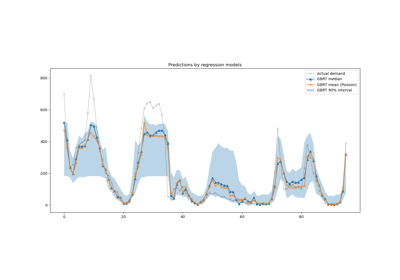
现在让我们定性地看看核模型和梯度提升树的预测,这些模型应该能够更好地建模特征之间的非线性交互。
gbrt.fit(X.iloc[train_0], y.iloc[train_0])
gbrt_predictions = gbrt.predict(X.iloc[test_0])

one_hot_poly_pipeline.fit(X.iloc[train_0], y.iloc[train_0])
one_hot_poly_predictions = one_hot_poly_pipeline.predict(X.iloc[test_0])

cyclic_spline_poly_pipeline.fit(X.iloc[train_0], y.iloc[train_0])
cyclic_spline_poly_predictions = cyclic_spline_poly_pipeline.predict(X.iloc[test_0])
我们再次放大测试集的最后 4 天。
last_hours = slice(-96, None)
fig, ax = plt.subplots(figsize=(12, 4))
fig.suptitle("Predictions by non-linear regression models")
ax.plot(
    y.iloc[test_0].values[last_hours],
    "x-",
    alpha=0.2,
    label="Actual demand",
    color="black",
)
ax.plot(
    gbrt_predictions[last_hours],
    "x-",
    label="Gradient Boosted Trees",
)
ax.plot(
    one_hot_poly_predictions[last_hours],
    "x-",
    label="One-hot + polynomial kernel",
)
ax.plot(
    cyclic_spline_poly_predictions[last_hours],
    "x-",
    label="Splines + polynomial kernel",
)
_ = ax.legend()
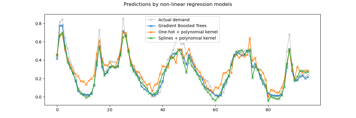
首先,请注意,树模型可以自然地建模非线性特征交互,因为默认情况下,决策树允许生长超过 2 层的深度。
在这里,我们可以观察到样条特征和非线性核的组合效果相当好,几乎可以与梯度提升回归树的准确性相媲美。
相反,独热编码时间特征在低秩核模型中表现不佳。特别是,它们比竞争模型显著高估了低需求小时。
我们还观察到,没有一个模型能够成功预测工作日高峰期的一些租赁峰值。可能需要额外的特征来进一步提高预测的准确性。例如,获取任意时间点的车队地理分布或因需要维修而无法使用的自行车比例可能会很有用。
最后,让我们使用真实需求与预测需求散点图,对这三个模型的预测误差进行更定量的观察。
from sklearn.metrics import PredictionErrorDisplay

fig, axes = plt.subplots(nrows=2, ncols=3, figsize=(13, 7), sharex=True, sharey="row")
fig.suptitle("Non-linear regression models", y=1.0)
predictions = [
    one_hot_poly_predictions,
    cyclic_spline_poly_predictions,
    gbrt_predictions,
]
labels = [
    "One hot +\npolynomial kernel",
    "Splines +\npolynomial kernel",
    "Gradient Boosted\nTrees",
]
plot_kinds = ["actual_vs_predicted", "residual_vs_predicted"]
for axis_idx, kind in enumerate(plot_kinds):
    for ax, pred, label in zip(axes[axis_idx], predictions, labels):
        disp = PredictionErrorDisplay.from_predictions(
            y_true=y.iloc[test_0],
            y_pred=pred,
            kind=kind,
            scatter_kwargs={"alpha": 0.3},
            ax=ax,
        )
        ax.set_xticks(np.linspace(0, 1, num=5))
        if axis_idx == 0:
            ax.set_yticks(np.linspace(0, 1, num=5))
            ax.legend(
                ["Best model", label],
                loc="upper center",
                bbox_to_anchor=(0.5, 1.3),
                ncol=2,
            )
        ax.set_aspect("equal", adjustable="box")
plt.show()
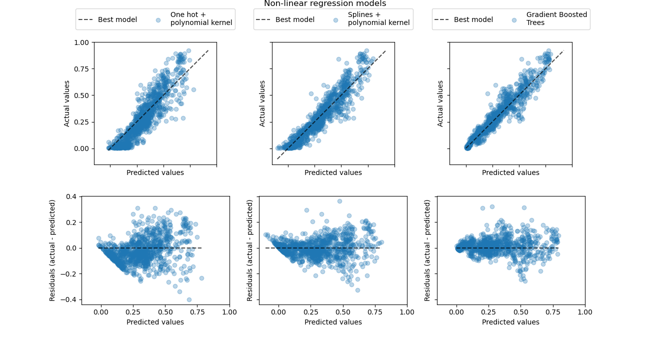
这种可视化证实了我们从上一张图中得出的结论。
所有模型都低估了高需求事件(工作日高峰期),但梯度提升模型低估程度稍小。梯度提升模型平均能很好地预测低需求事件,而独热多项式回归流水线似乎在该区域系统性地高估需求。总体而言,梯度提升树的预测比核模型的预测更接近对角线。
总结性说明#
我们注意到,对于核模型,通过使用更多的组件(更高秩的核近似),可以获得稍好的结果,但代价是更长的拟合和预测时间。对于较大的 n_components 值,独热编码特征的性能甚至可以与样条特征相匹配。
Nystroem + RidgeCV 回归器也可以被带有一到两个隐藏层的 MLPRegressor 替代,并且我们会得到相当相似的结果。
本案例研究中使用的数据集是按小时采样的。然而,循环样条特征可以以更细粒度的时间分辨率(例如,每分钟而不是每小时测量一次)高效地建模日内时间或周内时间,而无需引入更多特征。独热编码时间表示不具备这种灵活性。
最后,在本笔记本中,我们使用了 RidgeCV,因为它在计算方面非常高效。然而,它将目标变量建模为具有常数方差的高斯随机变量。对于正回归问题,使用泊松或伽马分布可能更有意义。这可以通过使用 GridSearchCV(TweedieRegressor(power=2), param_grid({"alpha": alphas})) 而不是 RidgeCV 来实现。
脚本总运行时间: (0 分钟 13.663 秒)
相关示例