注意
Go to the end to download the full example code or to run this example in your browser via JupyterLite or Binder.
异常值检测估计器的评估#
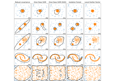
此示例比较了两种异常值检测算法,即 局部异常因子 (Local Outlier Factor, LOF) 和 孤立森林 (Isolation Forest, IForest),在 sklearn.datasets 中提供的真实世界数据集上的表现。目标是展示不同算法在不同数据集上表现良好,并对比它们的训练速度和对超参数的敏感性。
这些算法是在假设包含异常值的整个数据集上进行训练的(无标签)。
使用地面真值标签的知识计算 ROC 曲线,并使用
RocCurveDisplay显示。性能以 ROC-AUC 来评估。
# Authors: The scikit-learn developers
# SPDX-License-Identifier: BSD-3-Clause
数据集预处理和模型训练#
不同的异常值检测模型需要不同的预处理。在存在分类变量的情况下,OrdinalEncoder 通常是像 IsolationForest 这样的基于树的模型的一个很好的策略,而像 LocalOutlierFactor 这样的基于邻居的模型会受到序数编码引起的排序的影响。为了避免引入排序,应该使用 OneHotEncoder。
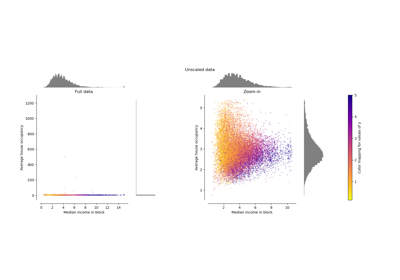
基于邻居的模型可能还需要对数值特征进行缩放(例如参见 重缩放对 k 近邻模型的影响)。在存在异常值的情况下,一个好的选择是使用 RobustScaler。
from sklearn.compose import ColumnTransformer
from sklearn.ensemble import IsolationForest
from sklearn.neighbors import LocalOutlierFactor
from sklearn.pipeline import make_pipeline
from sklearn.preprocessing import (
    OneHotEncoder,
    OrdinalEncoder,
    RobustScaler,
)


def make_estimator(name, categorical_columns=None, iforest_kw=None, lof_kw=None):
    """Create an outlier detection estimator based on its name."""
    if name == "LOF":
        outlier_detector = LocalOutlierFactor(**(lof_kw or {}))
        if categorical_columns is None:
            preprocessor = RobustScaler()
        else:
            preprocessor = ColumnTransformer(
                transformers=[("categorical", OneHotEncoder(), categorical_columns)],
                remainder=RobustScaler(),
            )
    else:  # name == "IForest"
        outlier_detector = IsolationForest(**(iforest_kw or {}))
        if categorical_columns is None:
            preprocessor = None
        else:
            ordinal_encoder = OrdinalEncoder(
                handle_unknown="use_encoded_value", unknown_value=-1
            )
            preprocessor = ColumnTransformer(
                transformers=[
                    ("categorical", ordinal_encoder, categorical_columns),
                ],
                remainder="passthrough",
            )

    return make_pipeline(preprocessor, outlier_detector)
以下 fit_predict 函数返回 X 的平均异常值分数。
from time import perf_counter


def fit_predict(estimator, X):
    tic = perf_counter()
    if estimator[-1].__class__.__name__ == "LocalOutlierFactor":
        estimator.fit(X)
        y_score = estimator[-1].negative_outlier_factor_
    else:  # "IsolationForest"
        y_score = estimator.fit(X).decision_function(X)
    toc = perf_counter()
    print(f"Duration for {model_name}: {toc - tic:.2f} s")
    return y_score
在示例的其余部分,我们按部分处理一个数据集。加载数据后,目标被修改为包含两个类:0 代表正常样本(inliers),1 代表异常样本(outliers)。由于 scikit-learn 文档的计算限制,一些数据集的样本大小通过分层 train_test_split 减少了。
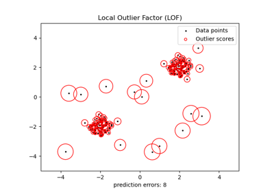
此外,我们设置 n_neighbors 以匹配预期的异常数量 expected_n_anomalies = n_samples * expected_anomaly_fraction。这是一个很好的启发式方法,只要异常值的比例不是非常低,原因是 n_neighbors 至少应大于样本数量较少的聚类中的样本数(参见 使用局部异常因子(LOF)进行异常值检测)。
KDDCup99 - SA 数据集#
Kddcup 99 数据集 是使用封闭网络和手动注入的攻击生成的。SA 数据集是通过简单地选择所有正常数据和大约 3% 的异常比例而获得的子集。
import numpy as np

from sklearn.datasets import fetch_kddcup99
from sklearn.model_selection import train_test_split

X, y = fetch_kddcup99(
    subset="SA", percent10=True, random_state=42, return_X_y=True, as_frame=True
)
y = (y != b"normal.").astype(np.int32)
X, _, y, _ = train_test_split(X, y, train_size=0.1, stratify=y, random_state=42)

n_samples, anomaly_frac = X.shape[0], y.mean()
print(f"{n_samples} datapoints with {y.sum()} anomalies ({anomaly_frac:.02%})")
10065 datapoints with 338 anomalies (3.36%)
SA 数据集包含 41 个特征,其中 3 个是分类特征:“protocol_type”、“service” 和 “flag”。
y_true = {}
y_score = {"LOF": {}, "IForest": {}}
model_names = ["LOF", "IForest"]
cat_columns = ["protocol_type", "service", "flag"]

y_true["KDDCup99 - SA"] = y
for model_name in model_names:
    model = make_estimator(
        name=model_name,
        categorical_columns=cat_columns,
        lof_kw={"n_neighbors": int(n_samples * anomaly_frac)},
        iforest_kw={"random_state": 42},
    )
    y_score[model_name]["KDDCup99 - SA"] = fit_predict(model, X)
Duration for LOF: 2.15 s
Duration for IForest: 0.27 s
森林覆盖类型数据集#
森林覆盖类型数据集 是一个多类数据集,目标是给定森林地块中的主要树种。它包含 54 个特征,其中一些(“Wilderness_Area” 和 “Soil_Type”)已经被二元编码。虽然最初是作为分类任务,但可以将标签为 2 的样本视为正常样本,将标签为 4 的样本视为异常样本。
from sklearn.datasets import fetch_covtype

X, y = fetch_covtype(return_X_y=True, as_frame=True)
s = (y == 2) + (y == 4)
X = X.loc[s]
y = y.loc[s]
y = (y != 2).astype(np.int32)

X, _, y, _ = train_test_split(X, y, train_size=0.05, stratify=y, random_state=42)
X_forestcover = X  # save X for later use

n_samples, anomaly_frac = X.shape[0], y.mean()
print(f"{n_samples} datapoints with {y.sum()} anomalies ({anomaly_frac:.02%})")
14302 datapoints with 137 anomalies (0.96%)
y_true["forestcover"] = y
for model_name in model_names:
    model = make_estimator(
        name=model_name,
        lof_kw={"n_neighbors": int(n_samples * anomaly_frac)},
        iforest_kw={"random_state": 42},
    )
    y_score[model_name]["forestcover"] = fit_predict(model, X)
Duration for LOF: 1.96 s
Duration for IForest: 0.22 s
Ames Housing 数据集#
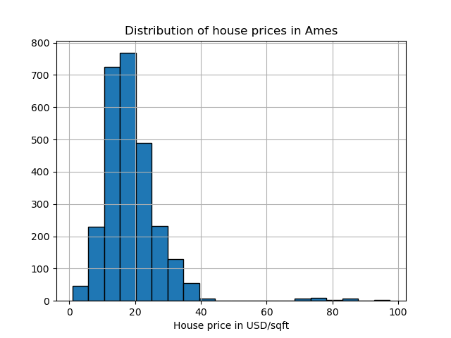
Ames housing 数据集 最初是一个回归数据集,目标是爱荷华州 Ames 房屋的销售价格。在这里,我们将其转换为异常值检测问题,将价格超过 70 美元/平方英尺的房屋视为异常值。为了使问题更容易,我们去除了价格在 40 到 70 美元/平方英尺之间的中间价格。
import matplotlib.pyplot as plt

from sklearn.datasets import fetch_openml

X, y = fetch_openml(name="ames_housing", version=1, return_X_y=True, as_frame=True)
y = y.div(X["Lot_Area"])

# None values in pandas 1.5.1 were mapped to np.nan in pandas 2.0.1
X["Misc_Feature"] = X["Misc_Feature"].cat.add_categories("NoInfo").fillna("NoInfo")
X["Mas_Vnr_Type"] = X["Mas_Vnr_Type"].cat.add_categories("NoInfo").fillna("NoInfo")

X.drop(columns="Lot_Area", inplace=True)
mask = (y < 40) | (y > 70)
X = X.loc[mask]
y = y.loc[mask]
y.hist(bins=20, edgecolor="black")
plt.xlabel("House price in USD/sqft")
_ = plt.title("Distribution of house prices in Ames")
y = (y > 70).astype(np.int32)

n_samples, anomaly_frac = X.shape[0], y.mean()
print(f"{n_samples} datapoints with {y.sum()} anomalies ({anomaly_frac:.02%})")
2714 datapoints with 30 anomalies (1.11%)
该数据集包含 46 个分类特征。在这种情况下,使用 make_column_selector 来查找它们比手动传递列表更容易。
from sklearn.compose import make_column_selector as selector

categorical_columns_selector = selector(dtype_include="category")
cat_columns = categorical_columns_selector(X)

y_true["ames_housing"] = y
for model_name in model_names:
    model = make_estimator(
        name=model_name,
        categorical_columns=cat_columns,
        lof_kw={"n_neighbors": int(n_samples * anomaly_frac)},
        iforest_kw={"random_state": 42},
    )
    y_score[model_name]["ames_housing"] = fit_predict(model, X)
Duration for LOF: 0.85 s
Duration for IForest: 0.21 s
心电图数据集#
心电图数据集 是胎儿心电图的多类数据集,类别是胎儿心率(FHR)模式,用 1 到 10 的标签编码。在这里,我们将类别 3(少数类)设置为代表异常值。它包含 30 个数值特征,其中一些是二元编码的,一些是连续的。
X, y = fetch_openml(name="cardiotocography", version=1, return_X_y=True, as_frame=False)
X_cardiotocography = X  # save X for later use
s = y == "3"
y = s.astype(np.int32)

n_samples, anomaly_frac = X.shape[0], y.mean()
print(f"{n_samples} datapoints with {y.sum()} anomalies ({anomaly_frac:.02%})")
2126 datapoints with 53 anomalies (2.49%)
y_true["cardiotocography"] = y
for model_name in model_names:
    model = make_estimator(
        name=model_name,
        lof_kw={"n_neighbors": int(n_samples * anomaly_frac)},
        iforest_kw={"random_state": 42},
    )
    y_score[model_name]["cardiotocography"] = fit_predict(model, X)
Duration for LOF: 0.06 s
Duration for IForest: 0.14 s
绘图并解释结果#
算法性能与在低假阳性率(FPR)值下真阳性率(TPR)的表现相关。最佳算法的曲线位于图的左上角,曲线下面积(AUC)接近 1。对角虚线代表异常值和正常样本的随机分类。
import math

from sklearn.metrics import RocCurveDisplay

cols = 2
pos_label = 0  # mean 0 belongs to positive class
datasets_names = y_true.keys()
rows = math.ceil(len(datasets_names) / cols)

fig, axs = plt.subplots(nrows=rows, ncols=cols, squeeze=False, figsize=(10, rows * 4))

for ax, dataset_name in zip(axs.ravel(), datasets_names):
    for model_idx, model_name in enumerate(model_names):
        display = RocCurveDisplay.from_predictions(
            y_true[dataset_name],
            y_score[model_name][dataset_name],
            pos_label=pos_label,
            name=model_name,
            ax=ax,
            plot_chance_level=(model_idx == len(model_names) - 1),
            chance_level_kw={"linestyle": ":"},
        )
    ax.set_title(dataset_name)
_ = plt.tight_layout(pad=2.0)  # spacing between subplots
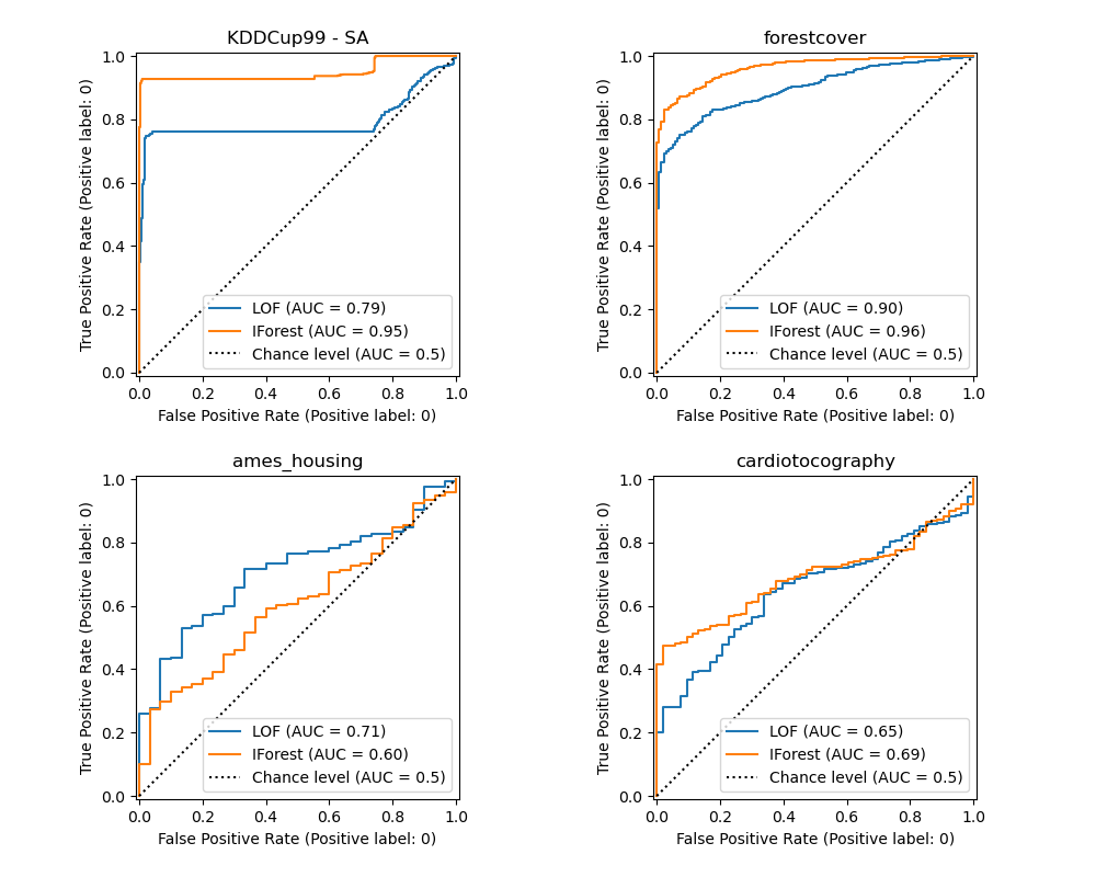
我们观察到,一旦调整了邻居数量,LOF 和 IForest 在 forestcover 和 cardiotocography 数据集上的 ROC AUC 方面表现相似。对于 SA 数据集,IForest 的分数稍好,而 LOF 在 Ames housing 数据集上的表现明显优于 IForest。
然而,请记住,在样本数量较多的数据集上,孤立森林的训练速度通常比 LOF 快得多。LOF 需要计算成对距离来找到最近邻居,这在观测数量方面具有二次复杂度。这使得该方法在大型数据集上可能难以应用。
消融研究#
在本节中,我们探讨了超参数 n_neighbors 和数值变量缩放选择对 LOF 模型的影响。在这里,我们使用 森林覆盖类型数据集,因为二元编码的类别引入了欧几里得距离在 0 和 1 之间的自然尺度。我们希望使用一种缩放方法,避免赋予非二元特征特权,并且对异常值足够鲁棒,以便寻找异常值的任务不会变得过于困难。
X = X_forestcover
y = y_true["forestcover"]

n_samples = X.shape[0]
n_neighbors_list = (n_samples * np.array([0.2, 0.02, 0.01, 0.001])).astype(np.int32)
model = make_pipeline(RobustScaler(), LocalOutlierFactor())

linestyles = ["solid", "dashed", "dashdot", ":", (5, (10, 3))]

fig, ax = plt.subplots()
for model_idx, (linestyle, n_neighbors) in enumerate(zip(linestyles, n_neighbors_list)):
    model.set_params(localoutlierfactor__n_neighbors=n_neighbors)
    model.fit(X)
    y_score = model[-1].negative_outlier_factor_
    display = RocCurveDisplay.from_predictions(
        y,
        y_score,
        pos_label=pos_label,
        name=f"n_neighbors = {n_neighbors}",
        ax=ax,
        plot_chance_level=(model_idx == len(n_neighbors_list) - 1),
        chance_level_kw={"linestyle": (0, (1, 10))},
        curve_kwargs=dict(linestyle=linestyle, linewidth=2),
    )
_ = ax.set_title("RobustScaler with varying n_neighbors\non forestcover dataset")
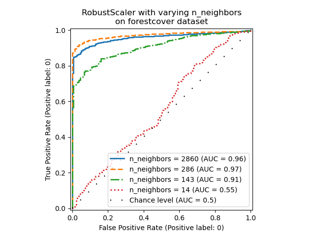
我们观察到邻居数量对模型性能有很大影响。如果可以访问(至少部分)地面真值标签,那么相应地调整 n_neighbors 非常重要。一个方便的方法是探索与预期污染程度数量级相同的 n_neighbors 值。
from sklearn.preprocessing import MinMaxScaler, SplineTransformer, StandardScaler

preprocessor_list = [
    None,
    RobustScaler(),
    StandardScaler(),
    MinMaxScaler(),
    SplineTransformer(),
]
expected_anomaly_fraction = 0.02
lof = LocalOutlierFactor(n_neighbors=int(n_samples * expected_anomaly_fraction))

fig, ax = plt.subplots()
for model_idx, (linestyle, preprocessor) in enumerate(
    zip(linestyles, preprocessor_list)
):
    model = make_pipeline(preprocessor, lof)
    model.fit(X)
    y_score = model[-1].negative_outlier_factor_
    display = RocCurveDisplay.from_predictions(
        y,
        y_score,
        pos_label=pos_label,
        name=str(preprocessor).split("(")[0],
        ax=ax,
        plot_chance_level=(model_idx == len(preprocessor_list) - 1),
        chance_level_kw={"linestyle": (0, (1, 10))},
        curve_kwargs=dict(linestyle=linestyle, linewidth=2),
    )
_ = ax.set_title("Fixed n_neighbors with varying preprocessing\non forestcover dataset")
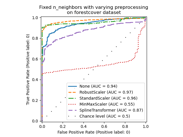
一方面,RobustScaler 默认使用四分位距(IQR)独立缩放每个特征,IQR 是数据第 25 个百分位数和第 75 个百分位数之间的范围。它通过减去中位数来中心化数据,然后除以 IQR 来缩放数据。IQR 对异常值具有鲁棒性:中位数和四分位距受极端值的影响小于范围、均值和标准差。此外,与 StandardScaler 不同,RobustScaler 不会压缩边缘异常值。
另一方面,MinMaxScaler 独立缩放每个特征,使其范围映射到零到一的范围内。如果数据中存在异常值,它们可能会使数据偏向最小值或最大值,导致数据分布完全不同,并且边缘异常值很大:所有非异常值可能会因此几乎崩溃在一起。
我们还评估了根本不进行预处理(通过向管道传递 None)、StandardScaler 和 SplineTransformer。请参阅它们各自的文档以获取更多详细信息。
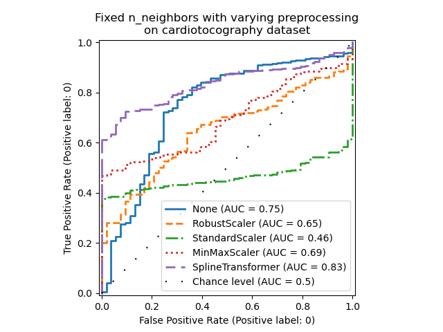
请注意,最佳预处理取决于数据集,如下所示。
X = X_cardiotocography
y = y_true["cardiotocography"]

n_samples, expected_anomaly_fraction = X.shape[0], 0.025
lof = LocalOutlierFactor(n_neighbors=int(n_samples * expected_anomaly_fraction))

fig, ax = plt.subplots()
for model_idx, (linestyle, preprocessor) in enumerate(
    zip(linestyles, preprocessor_list)
):
    model = make_pipeline(preprocessor, lof)
    model.fit(X)
    y_score = model[-1].negative_outlier_factor_
    display = RocCurveDisplay.from_predictions(
        y,
        y_score,
        pos_label=pos_label,
        name=str(preprocessor).split("(")[0],
        ax=ax,
        plot_chance_level=(model_idx == len(preprocessor_list) - 1),
        chance_level_kw={"linestyle": (0, (1, 10))},
        curve_kwargs=dict(linestyle=linestyle, linewidth=2),
    )
ax.set_title(
    "Fixed n_neighbors with varying preprocessing\non cardiotocography dataset"
)
plt.show()
脚本总运行时间: (1 minutes 5.097 seconds)
相关示例