MNIST 上的多层感知器 (MLP) 权重可视化#

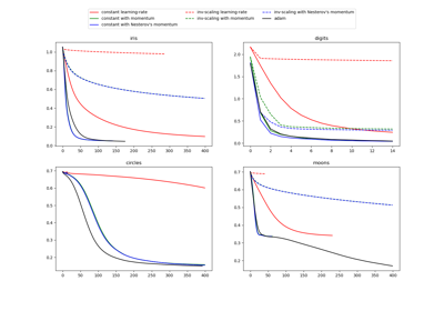
有时查看神经网络的学习系数可以深入了解学习行为。例如，如果权重看起来没有结构，也许有些权重根本没有使用，或者如果存在非常大的系数，也许正则化太低或学习率太高。

此示例演示如何在 MNIST 数据集上训练的 MLPClassifier 中绘制一些第一层权重。

输入数据由 28x28 像素的手写数字组成，导致数据集中有 784 个特征。因此，第一层权重矩阵的形状为 (784, hidden_layer_sizes[0])。因此，我们可以将权重矩阵的一列可视化为 28x28 像素的图像。

为了使示例运行更快，我们使用非常少的隐藏单元，并且只训练很短的时间。更长的训练将导致权重具有更平滑的空间外观。此示例将抛出一个警告，因为它没有收敛，在这种情况下，这是我们想要的，因为我们在持续集成基础设施上构建此文档时存在资源使用限制。

Iteration 1, loss = 0.44139186
Iteration 2, loss = 0.19174891
Iteration 3, loss = 0.13983521
Iteration 4, loss = 0.11378556
Iteration 5, loss = 0.09443967
Iteration 6, loss = 0.07846529
Iteration 7, loss = 0.06506307
Iteration 8, loss = 0.05534985
Training set score: 0.986429
Test set score: 0.953061

# Authors: The scikit-learn developers
# SPDX-License-Identifier: BSD-3-Clause

import warnings

import matplotlib.pyplot as plt

from sklearn.datasets import fetch_openml
from sklearn.exceptions import ConvergenceWarning
from sklearn.model_selection import train_test_split
from sklearn.neural_network import MLPClassifier

# Load data from https://www.openml.org/d/554
X, y = fetch_openml("mnist_784", version=1, return_X_y=True, as_frame=False)
X = X / 255.0

# Split data into train partition and test partition
X_train, X_test, y_train, y_test = train_test_split(X, y, random_state=0, test_size=0.7)

mlp = MLPClassifier(
    hidden_layer_sizes=(40,),
    max_iter=8,
    alpha=1e-4,
    solver="sgd",
    verbose=10,
    random_state=1,
    learning_rate_init=0.2,
)

# this example won't converge because of resource usage constraints on
# our Continuous Integration infrastructure, so we catch the warning and
# ignore it here
with warnings.catch_warnings():
    warnings.filterwarnings("ignore", category=ConvergenceWarning, module="sklearn")
    mlp.fit(X_train, y_train)

print("Training set score: %f" % mlp.score(X_train, y_train))
print("Test set score: %f" % mlp.score(X_test, y_test))

fig, axes = plt.subplots(4, 4)
# use global min / max to ensure all weights are shown on the same scale
vmin, vmax = mlp.coefs_[0].min(), mlp.coefs_[0].max()
for coef, ax in zip(mlp.coefs_[0].T, axes.ravel()):
    ax.matshow(coef.reshape(28, 28), cmap=plt.cm.gray, vmin=0.5 * vmin, vmax=0.5 * vmax)
    ax.set_xticks(())
    ax.set_yticks(())

plt.show()

脚本总运行时间：（0 分钟 10.089 秒）