Swiss Roll 和 Swiss-Hole 降维#

本笔记旨在比较两种流行的非线性降维技术，t-SNE（T 分布式随机邻近嵌入）和 LLE（局部线性嵌入），在经典的 Swiss Roll 数据集上的表现。然后，我们将探讨它们如何处理在数据中添加一个“洞”（Swiss-Hole）。

# Authors: The scikit-learn developers
# SPDX-License-Identifier: BSD-3-Clause

Swiss Roll#

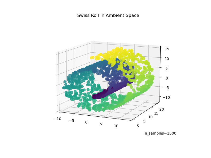
我们首先生成 Swiss Roll 数据集。

import matplotlib.pyplot as plt

from sklearn import datasets, manifold

sr_points, sr_color = datasets.make_swiss_roll(n_samples=1500, random_state=0)

现在，让我们看看我们的数据

fig = plt.figure(figsize=(8, 6))
ax = fig.add_subplot(111, projection="3d")
fig.add_axes(ax)
ax.scatter(
    sr_points[:, 0], sr_points[:, 1], sr_points[:, 2], c=sr_color, s=50, alpha=0.8
)
ax.set_title("Swiss Roll in Ambient Space")
ax.view_init(azim=-66, elev=12)
_ = ax.text2D(0.8, 0.05, s="n_samples=1500", transform=ax.transAxes)

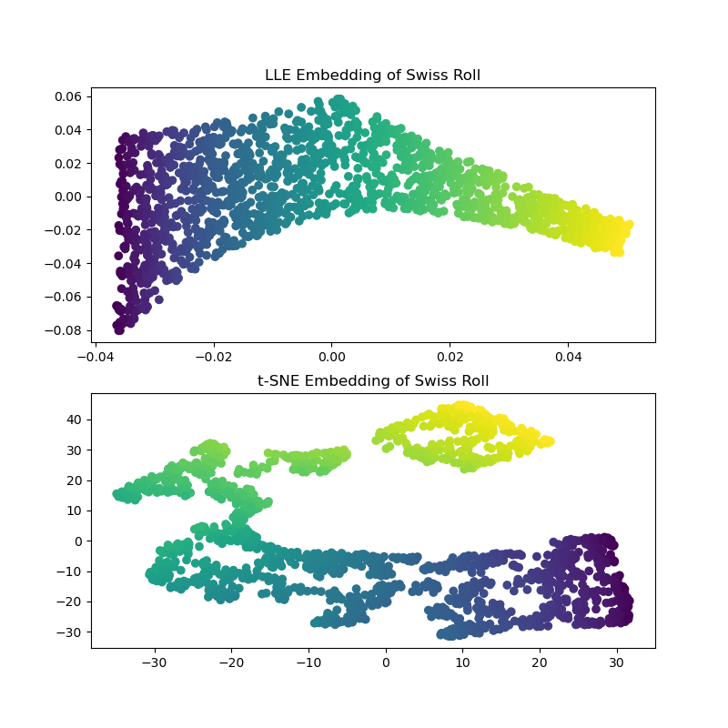
计算 LLE 和 t-SNE 嵌入，我们发现 LLE 似乎能非常有效地展开 Swiss Roll。另一方面，t-SNE 能够保留数据的总体结构，但对原始数据的连续性表示不佳。相反，它似乎不必要地将某些部分点聚集在一起。

sr_lle, sr_err = manifold.locally_linear_embedding(
    sr_points, n_neighbors=12, n_components=2
)

sr_tsne = manifold.TSNE(n_components=2, perplexity=40, random_state=0).fit_transform(
    sr_points
)

fig, axs = plt.subplots(figsize=(8, 8), nrows=2)
axs[0].scatter(sr_lle[:, 0], sr_lle[:, 1], c=sr_color)
axs[0].set_title("LLE Embedding of Swiss Roll")
axs[1].scatter(sr_tsne[:, 0], sr_tsne[:, 1], c=sr_color)
_ = axs[1].set_title("t-SNE Embedding of Swiss Roll")

LLE Embedding of Swiss Roll, t-SNE Embedding of Swiss Roll

注意

LLE 似乎拉伸了 Swiss Roll 中心（紫色）的点。然而，我们观察到这仅仅是数据生成方式的副产品。卷中心附近的点密度更高，这最终影响了 LLE 在较低维度中重建数据的方式。

Swiss-Hole#

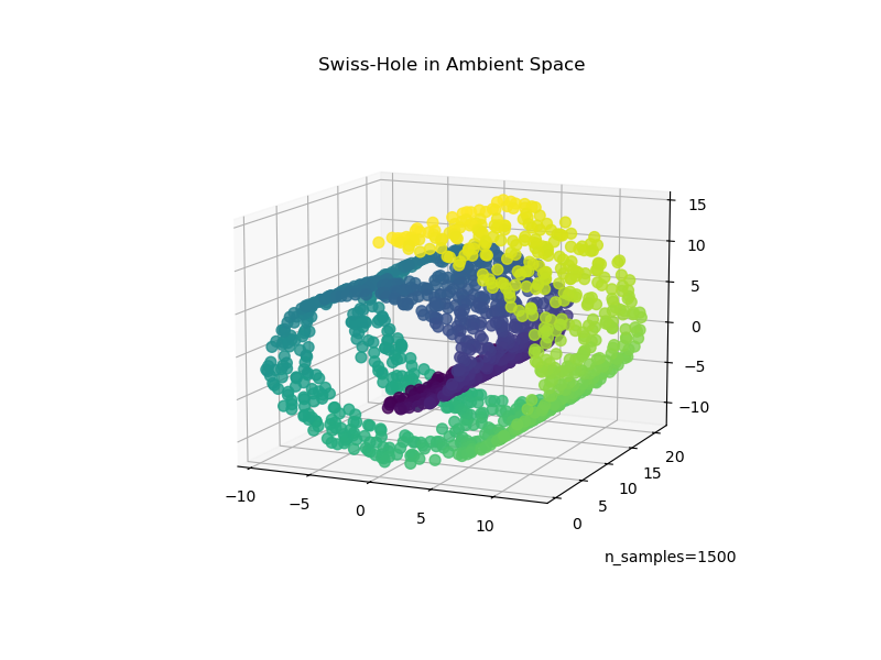
现在让我们看看当我们向数据添加一个洞时，这两种算法如何应对。首先，我们生成 Swiss-Hole 数据集并绘制它

sh_points, sh_color = datasets.make_swiss_roll(
    n_samples=1500, hole=True, random_state=0
)

fig = plt.figure(figsize=(8, 6))
ax = fig.add_subplot(111, projection="3d")
fig.add_axes(ax)
ax.scatter(
    sh_points[:, 0], sh_points[:, 1], sh_points[:, 2], c=sh_color, s=50, alpha=0.8
)
ax.set_title("Swiss-Hole in Ambient Space")
ax.view_init(azim=-66, elev=12)
_ = ax.text2D(0.8, 0.05, s="n_samples=1500", transform=ax.transAxes)

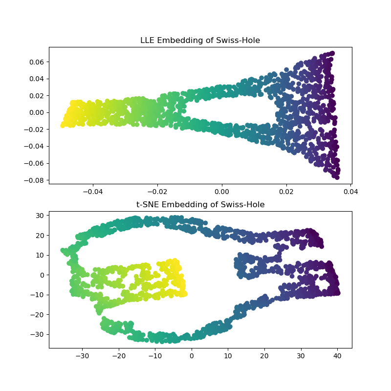
计算 LLE 和 t-SNE 嵌入，我们得到了与 Swiss Roll 相似的结果。LLE 非常熟练地展开了数据，甚至保留了洞。t-SNE 再次将点的一部分聚集在一起，但我们注意到它保留了原始数据的总体拓扑结构。

sh_lle, sh_err = manifold.locally_linear_embedding(
    sh_points, n_neighbors=12, n_components=2
)

sh_tsne = manifold.TSNE(
    n_components=2, perplexity=40, init="random", random_state=0
).fit_transform(sh_points)

fig, axs = plt.subplots(figsize=(8, 8), nrows=2)
axs[0].scatter(sh_lle[:, 0], sh_lle[:, 1], c=sh_color)
axs[0].set_title("LLE Embedding of Swiss-Hole")
axs[1].scatter(sh_tsne[:, 0], sh_tsne[:, 1], c=sh_color)
_ = axs[1].set_title("t-SNE Embedding of Swiss-Hole")

LLE Embedding of Swiss-Hole, t-SNE Embedding of Swiss-Hole

总结性评论#

我们注意到 t-SNE 受益于测试更多参数组合。通过更好地调整这些参数，可能会获得更好的结果。

我们观察到，正如在“手写数字流形学习”示例中所见，t-SNE 通常在真实世界数据上的表现优于 LLE。

脚本总运行时间： (0 分钟 16.974 秒)

Swiss Roll 和 Swiss-Hole 降维#

Swiss Roll#

Swiss-Hole#

总结性评论#

本页