使用成本复杂度剪枝对决策树进行后剪枝#

DecisionTreeClassifier 提供了诸如 min_samples_leaf 和 max_depth 等参数来防止树过度拟合。成本复杂度剪枝提供了另一种控制树大小的选项。在 DecisionTreeClassifier 中，这种剪枝技术由成本复杂度参数 ccp_alpha 参数化。更大的 ccp_alpha 值会增加剪枝的节点数。在这里，我们只展示 ccp_alpha 对树正则化的影响，以及如何根据验证分数选择 ccp_alpha。

有关剪枝的详细信息，请参阅最小成本复杂度剪枝。

# Authors: The scikit-learn developers
# SPDX-License-Identifier: BSD-3-Clause

import matplotlib.pyplot as plt

from sklearn.datasets import load_breast_cancer
from sklearn.model_selection import train_test_split
from sklearn.tree import DecisionTreeClassifier

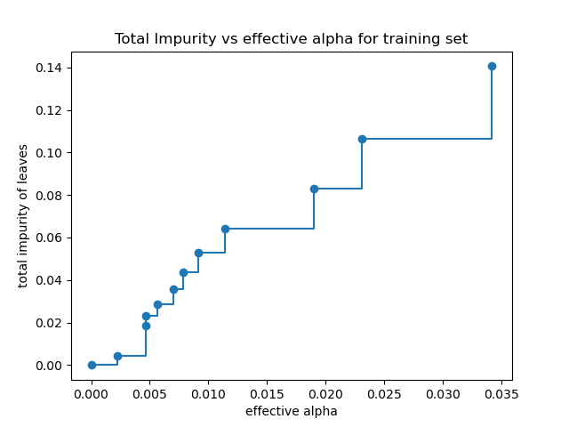
叶子总杂质与剪枝树的有效 alpha 值#

最小成本复杂度剪枝递归地找到具有“最弱链接”的节点。最弱链接的特征是有效 alpha 值，其中具有最小有效 alpha 值的节点首先被剪枝。为了了解哪些 ccp_alpha 值可能合适，scikit-learn 提供了 DecisionTreeClassifier.cost_complexity_pruning_path，它返回剪枝过程中每一步的有效 alpha 值和相应的叶子总杂质。随着 alpha 值的增加，更多的树被剪枝，这增加了其叶子的总杂质。

X, y = load_breast_cancer(return_X_y=True)
X_train, X_test, y_train, y_test = train_test_split(X, y, random_state=0)

clf = DecisionTreeClassifier(random_state=0)
path = clf.cost_complexity_pruning_path(X_train, y_train)
ccp_alphas, impurities = path.ccp_alphas, path.impurities

在下面的图中，移除了最大有效 alpha 值，因为它是一棵只有一个节点的普通树。

fig, ax = plt.subplots()
ax.plot(ccp_alphas[:-1], impurities[:-1], marker="o", drawstyle="steps-post")
ax.set_xlabel("effective alpha")
ax.set_ylabel("total impurity of leaves")
ax.set_title("Total Impurity vs effective alpha for training set")

Total Impurity vs effective alpha for training set

Text(0.5, 1.0, 'Total Impurity vs effective alpha for training set')

接下来，我们使用有效 alpha 值训练决策树。ccp_alphas 中的最后一个值是剪枝整个树的 alpha 值，留下树 clfs[-1] 只有一个节点。

clfs = []
for ccp_alpha in ccp_alphas:
    clf = DecisionTreeClassifier(random_state=0, ccp_alpha=ccp_alpha)
    clf.fit(X_train, y_train)
    clfs.append(clf)
print(
    "Number of nodes in the last tree is: {} with ccp_alpha: {}".format(
        clfs[-1].tree_.node_count, ccp_alphas[-1]
    )
)

Number of nodes in the last tree is: 1 with ccp_alpha: 0.3272984419327777

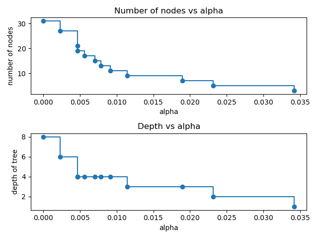
对于本例的其余部分，我们移除了 clfs 和 ccp_alphas 中的最后一个元素，因为它是一棵只有一个节点的普通树。在这里，我们展示了节点数和树深度随着 alpha 值的增加而减少。

clfs = clfs[:-1]
ccp_alphas = ccp_alphas[:-1]

node_counts = [clf.tree_.node_count for clf in clfs]
depth = [clf.tree_.max_depth for clf in clfs]
fig, ax = plt.subplots(2, 1)
ax[0].plot(ccp_alphas, node_counts, marker="o", drawstyle="steps-post")
ax[0].set_xlabel("alpha")
ax[0].set_ylabel("number of nodes")
ax[0].set_title("Number of nodes vs alpha")
ax[1].plot(ccp_alphas, depth, marker="o", drawstyle="steps-post")
ax[1].set_xlabel("alpha")
ax[1].set_ylabel("depth of tree")
ax[1].set_title("Depth vs alpha")
fig.tight_layout()

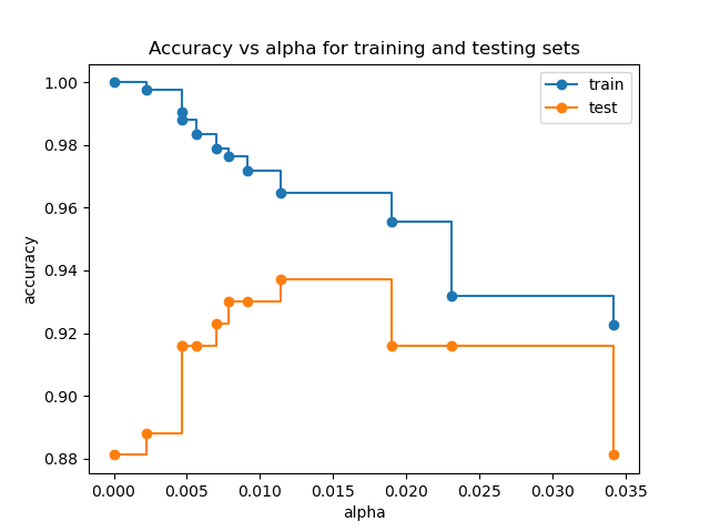
Number of nodes vs alpha, Depth vs alpha

训练集和测试集的准确性与 alpha 值#

当 ccp_alpha 设置为零并保持 DecisionTreeClassifier 的其他默认参数时，树会过度拟合，导致 100% 的训练准确性和 88% 的测试准确性。随着 alpha 值的增加，更多的树被剪枝，从而创建了一个泛化能力更好的决策树。在这个例子中，设置 ccp_alpha=0.015 可以使测试准确性最大化。

train_scores = [clf.score(X_train, y_train) for clf in clfs]
test_scores = [clf.score(X_test, y_test) for clf in clfs]

fig, ax = plt.subplots()
ax.set_xlabel("alpha")
ax.set_ylabel("accuracy")
ax.set_title("Accuracy vs alpha for training and testing sets")
ax.plot(ccp_alphas, train_scores, marker="o", label="train", drawstyle="steps-post")
ax.plot(ccp_alphas, test_scores, marker="o", label="test", drawstyle="steps-post")
ax.legend()
plt.show()

Accuracy vs alpha for training and testing sets

脚本总运行时间： (0 分钟 0.380 秒)

使用成本复杂度剪枝对决策树进行后剪枝#

叶子总杂质与剪枝树的有效 alpha 值#

训练集和测试集的准确性与 alpha 值#

本页