使用 IterativeImputer 的变体来插补缺失值#

IterativeImputer 类非常灵活 - 它可以与各种估计器一起使用来执行循环回归，依次将每个变量视为输出。

在本例中，我们比较了一些用于使用 IterativeImputer 插补缺失特征的估计器

BayesianRidge：正则化线性回归
RandomForestRegressor：随机树森林回归
make_pipeline (Nystroem, Ridge)：一个包含 2 次多项式核展开和正则化线性回归的管道
KNeighborsRegressor：可与其他 KNN 插补方法相媲美

特别值得注意的是 IterativeImputer 能够模拟 missForest 的行为，missForest 是 R 中流行的插补包。

请注意，KNeighborsRegressor 与 KNN 插补不同，后者通过使用考虑缺失值的距离度量从具有缺失值的样本中学习，而不是插补它们。

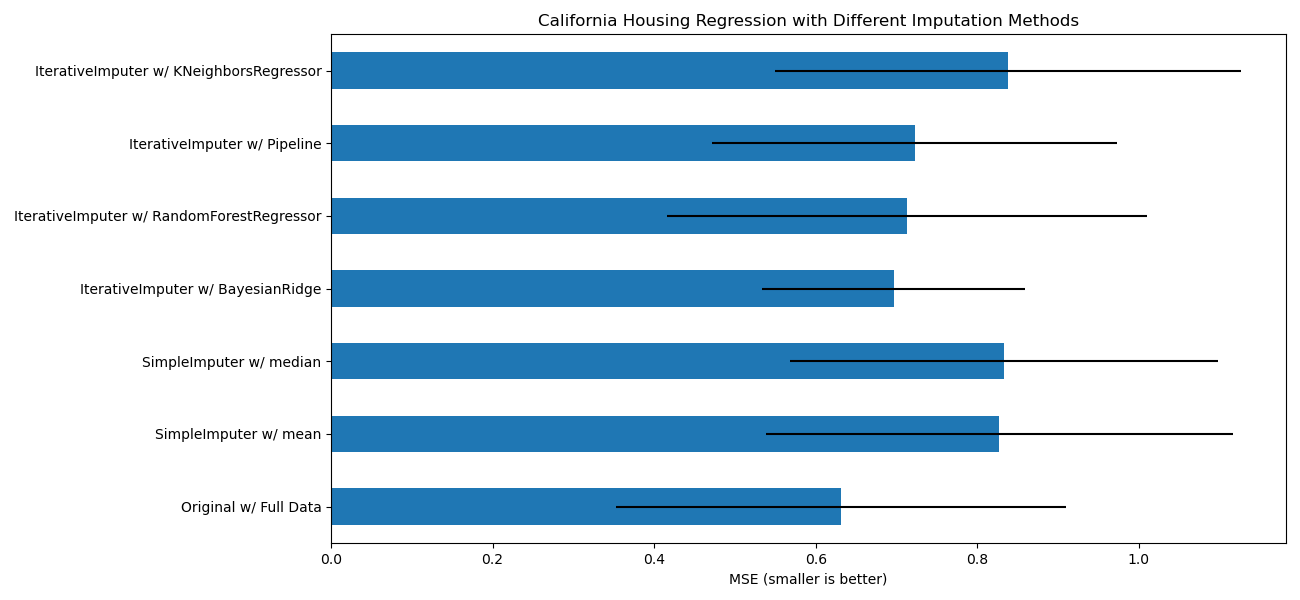
目标是比较不同的估计器，以了解在使用 BayesianRidge 估计器对加州住房数据集进行插补时，哪个估计器最适合 IterativeImputer，其中每行随机删除一个值。

对于这种特定的缺失值模式，我们看到 BayesianRidge 和 RandomForestRegressor 提供了最佳结果。

应该指出，一些估计器，如 HistGradientBoostingRegressor 可以原生处理缺失特征，并且通常建议使用它们而不是构建包含复杂且昂贵的缺失值插补策略的管道。

California Housing Regression with Different Imputation Methods

# Authors: The scikit-learn developers
# SPDX-License-Identifier: BSD-3-Clause

import matplotlib.pyplot as plt
import numpy as np
import pandas as pd

from sklearn.datasets import fetch_california_housing
from sklearn.ensemble import RandomForestRegressor

# To use this experimental feature, we need to explicitly ask for it:
from sklearn.experimental import enable_iterative_imputer  # noqa: F401
from sklearn.impute import IterativeImputer, SimpleImputer
from sklearn.kernel_approximation import Nystroem
from sklearn.linear_model import BayesianRidge, Ridge
from sklearn.model_selection import cross_val_score
from sklearn.neighbors import KNeighborsRegressor
from sklearn.pipeline import make_pipeline
from sklearn.preprocessing import RobustScaler

N_SPLITS = 5

X_full, y_full = fetch_california_housing(return_X_y=True)
# ~2k samples is enough for the purpose of the example.
# Remove the following two lines for a slower run with different error bars.
X_full = X_full[::10]
y_full = y_full[::10]
n_samples, n_features = X_full.shape


def compute_score_for(X, y, imputer=None):
    # We scale data before imputation and training a target estimator,
    # because our target estimator and some of the imputers assume
    # that the features have similar scales.
    if imputer is None:
        estimator = make_pipeline(RobustScaler(), BayesianRidge())
    else:
        estimator = make_pipeline(RobustScaler(), imputer, BayesianRidge())
    return cross_val_score(
        estimator, X, y, scoring="neg_mean_squared_error", cv=N_SPLITS
    )


# Estimate the score on the entire dataset, with no missing values
score_full_data = pd.DataFrame(
    compute_score_for(X_full, y_full),
    columns=["Full Data"],
)

# Add a single missing value to each row
rng = np.random.RandomState(0)
X_missing = X_full.copy()
y_missing = y_full
missing_samples = np.arange(n_samples)
missing_features = rng.choice(n_features, n_samples, replace=True)
X_missing[missing_samples, missing_features] = np.nan

# Estimate the score after imputation (mean and median strategies)
score_simple_imputer = pd.DataFrame()
for strategy in ("mean", "median"):
    score_simple_imputer[strategy] = compute_score_for(
        X_missing, y_missing, SimpleImputer(strategy=strategy)
    )

# Estimate the score after iterative imputation of the missing values
# with different estimators
named_estimators = [
    ("Bayesian Ridge", BayesianRidge()),
    (
        "Random Forest",
        RandomForestRegressor(
            # We tuned the hyperparameters of the RandomForestRegressor to get a good
            # enough predictive performance for a restricted execution time.
            n_estimators=5,
            max_depth=10,
            bootstrap=True,
            max_samples=0.5,
            n_jobs=2,
            random_state=0,
        ),
    ),
    (
        "Nystroem + Ridge",
        make_pipeline(
            Nystroem(kernel="polynomial", degree=2, random_state=0), Ridge(alpha=1e4)
        ),
    ),
    (
        "k-NN",
        KNeighborsRegressor(n_neighbors=10),
    ),
]
score_iterative_imputer = pd.DataFrame()
# Iterative imputer is sensitive to the tolerance and
# dependent on the estimator used internally.
# We tuned the tolerance to keep this example run with limited computational
# resources while not changing the results too much compared to keeping the
# stricter default value for the tolerance parameter.
tolerances = (1e-3, 1e-1, 1e-1, 1e-2)
for (name, impute_estimator), tol in zip(named_estimators, tolerances):
    score_iterative_imputer[name] = compute_score_for(
        X_missing,
        y_missing,
        IterativeImputer(
            random_state=0, estimator=impute_estimator, max_iter=40, tol=tol
        ),
    )

scores = pd.concat(
    [score_full_data, score_simple_imputer, score_iterative_imputer],
    keys=["Original", "SimpleImputer", "IterativeImputer"],
    axis=1,
)

# plot california housing results
fig, ax = plt.subplots(figsize=(13, 6))
means = -scores.mean()
errors = scores.std()
means.plot.barh(xerr=errors, ax=ax)
ax.set_title("California Housing Regression with Different Imputation Methods")
ax.set_xlabel("MSE (smaller is better)")
ax.set_yticks(np.arange(means.shape[0]))
ax.set_yticklabels([" w/ ".join(label) for label in means.index.tolist()])
plt.tight_layout(pad=1)
plt.show()

脚本总运行时间： (0 分钟 6.116 秒)

使用 IterativeImputer 的变体来插补缺失值#

本页