注意
转至末尾以下载完整示例代码或通过 JupyterLite 或 Binder 在浏览器中运行此示例。
平衡模型复杂度和交叉验证分数#
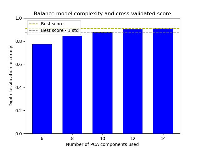
此示例演示如何通过在最佳准确率分数的 1 个标准差内找到一个合适的准确率,同时最大限度地减少 PCA 组件的数量,来平衡模型复杂度和交叉验证分数 [1]。它使用带有自定义 refit callable 的 GridSearchCV 来选择最佳模型。
该图显示了交叉验证分数和 PCA 组件数量之间的权衡。平衡情况是当 n_components=10 且 accuracy=0.88 时,这落在最佳准确率分数的 1 个标准差范围内。
参考文献#
# Authors: The scikit-learn developers
# SPDX-License-Identifier: BSD-3-Clause

import matplotlib.pyplot as plt
import numpy as np
import polars as pl

from sklearn.datasets import load_digits
from sklearn.decomposition import PCA
from sklearn.linear_model import LogisticRegression
from sklearn.model_selection import GridSearchCV, ShuffleSplit
from sklearn.pipeline import Pipeline
引言#
在调整超参数时,我们通常希望平衡模型复杂度和性能。“一标准误”规则是一种常用方法:选择性能在最佳模型性能的一个标准误范围内的最简单模型。这有助于通过在性能统计上与更复杂的模型相当时偏好更简单的模型来避免过拟合。
辅助函数#
我们定义了两个辅助函数
lower_bound: 计算可接受性能的阈值(最佳分数 - 1 个标准差)best_low_complexity: 选择 PCA 组件最少但超过此阈值的模型
def lower_bound(cv_results):
    """
    Calculate the lower bound within 1 standard deviation
    of the best `mean_test_scores`.

    Parameters
    ----------
    cv_results : dict of numpy(masked) ndarrays
        See attribute cv_results_ of `GridSearchCV`

    Returns
    -------
    float
        Lower bound within 1 standard deviation of the
        best `mean_test_score`.
    """
    best_score_idx = np.argmax(cv_results["mean_test_score"])

    return (
        cv_results["mean_test_score"][best_score_idx]
        - cv_results["std_test_score"][best_score_idx]
    )


def best_low_complexity(cv_results):
    """
    Balance model complexity with cross-validated score.

    Parameters
    ----------
    cv_results : dict of numpy(masked) ndarrays
        See attribute cv_results_ of `GridSearchCV`.

    Return
    ------
    int
        Index of a model that has the fewest PCA components
        while has its test score within 1 standard deviation of the best
        `mean_test_score`.
    """
    threshold = lower_bound(cv_results)
    candidate_idx = np.flatnonzero(cv_results["mean_test_score"] >= threshold)
    best_idx = candidate_idx[
        cv_results["param_reduce_dim__n_components"][candidate_idx].argmin()
    ]
    return best_idx
设置管道和参数网格#
我们创建一个包含两个步骤的管道
使用 PCA 进行降维
使用 LogisticRegression 进行分类
我们将搜索不同数量的 PCA 组件以找到最佳复杂度。
pipe = Pipeline(
    [
        ("reduce_dim", PCA(random_state=42)),
        ("classify", LogisticRegression(random_state=42, C=0.01, max_iter=1000)),
    ]
)

param_grid = {"reduce_dim__n_components": [6, 8, 10, 15, 20, 25, 35, 45, 55]}
使用 GridSearchCV 执行搜索#
我们使用 GridSearchCV 并将我们的自定义 best_low_complexity 函数作为 refit 参数。此函数将选择 PCA 组件最少但性能仍在最佳模型的一个标准差范围内的模型。
grid = GridSearchCV(
    pipe,
    # Use a non-stratified CV strategy to make sure that the inter-fold
    # standard deviation of the test scores is informative.
    cv=ShuffleSplit(n_splits=30, random_state=0),
    n_jobs=1,  # increase this on your machine to use more physical cores
    param_grid=param_grid,
    scoring="accuracy",
    refit=best_low_complexity,
    return_train_score=True,
)
加载 digits 数据集并拟合模型#
X, y = load_digits(return_X_y=True)
grid.fit(X, y)
可视化结果#
我们将创建一个条形图,显示不同数量 PCA 组件的测试分数,以及表示最佳分数和一标准差阈值的水平线。
n_components = grid.cv_results_["param_reduce_dim__n_components"]
test_scores = grid.cv_results_["mean_test_score"]

# Create a polars DataFrame for better data manipulation and visualization
results_df = pl.DataFrame(
    {
        "n_components": n_components,
        "mean_test_score": test_scores,
        "std_test_score": grid.cv_results_["std_test_score"],
        "mean_train_score": grid.cv_results_["mean_train_score"],
        "std_train_score": grid.cv_results_["std_train_score"],
        "mean_fit_time": grid.cv_results_["mean_fit_time"],
        "rank_test_score": grid.cv_results_["rank_test_score"],
    }
)

# Sort by number of components
results_df = results_df.sort("n_components")

# Calculate the lower bound threshold
lower = lower_bound(grid.cv_results_)

# Get the best model information
best_index_ = grid.best_index_
best_components = n_components[best_index_]
best_score = grid.cv_results_["mean_test_score"][best_index_]

# Add a column to mark the selected model
results_df = results_df.with_columns(
    pl.when(pl.col("n_components") == best_components)
    .then(pl.lit("Selected"))
    .otherwise(pl.lit("Regular"))
    .alias("model_type")
)

# Get the number of CV splits from the results
n_splits = sum(
    1
    for key in grid.cv_results_.keys()
    if key.startswith("split") and key.endswith("test_score")
)

# Extract individual scores for each split
test_scores = np.array(
    [
        [grid.cv_results_[f"split{i}_test_score"][j] for i in range(n_splits)]
        for j in range(len(n_components))
    ]
)
train_scores = np.array(
    [
        [grid.cv_results_[f"split{i}_train_score"][j] for i in range(n_splits)]
        for j in range(len(n_components))
    ]
)

# Calculate mean and std of test scores
mean_test_scores = np.mean(test_scores, axis=1)
std_test_scores = np.std(test_scores, axis=1)

# Find best score and threshold
best_mean_score = np.max(mean_test_scores)
threshold = best_mean_score - std_test_scores[np.argmax(mean_test_scores)]

# Create a single figure for visualization
fig, ax = plt.subplots(figsize=(12, 8))

# Plot individual points
for i, comp in enumerate(n_components):
    # Plot individual test points
    plt.scatter(
        [comp] * n_splits,
        test_scores[i],
        alpha=0.2,
        color="blue",
        s=20,
        label="Individual test scores" if i == 0 else "",
    )
    # Plot individual train points
    plt.scatter(
        [comp] * n_splits,
        train_scores[i],
        alpha=0.2,
        color="green",
        s=20,
        label="Individual train scores" if i == 0 else "",
    )

# Plot mean lines with error bands
plt.plot(
    n_components,
    np.mean(test_scores, axis=1),
    "-",
    color="blue",
    linewidth=2,
    label="Mean test score",
)
plt.fill_between(
    n_components,
    np.mean(test_scores, axis=1) - np.std(test_scores, axis=1),
    np.mean(test_scores, axis=1) + np.std(test_scores, axis=1),
    alpha=0.15,
    color="blue",
)

plt.plot(
    n_components,
    np.mean(train_scores, axis=1),
    "-",
    color="green",
    linewidth=2,
    label="Mean train score",
)
plt.fill_between(
    n_components,
    np.mean(train_scores, axis=1) - np.std(train_scores, axis=1),
    np.mean(train_scores, axis=1) + np.std(train_scores, axis=1),
    alpha=0.15,
    color="green",
)

# Add threshold lines
plt.axhline(
    best_mean_score,
    color="#9b59b6",  # Purple
    linestyle="--",
    label="Best score",
    linewidth=2,
)
plt.axhline(
    threshold,
    color="#e67e22",  # Orange
    linestyle="--",
    label="Best score - 1 std",
    linewidth=2,
)

# Highlight selected model
plt.axvline(
    best_components,
    color="#9b59b6",  # Purple
    alpha=0.2,
    linewidth=8,
    label="Selected model",
)

# Set titles and labels
plt.xlabel("Number of PCA components", fontsize=12)
plt.ylabel("Score", fontsize=12)
plt.title("Model Selection: Balancing Complexity and Performance", fontsize=14)
plt.grid(True, linestyle="--", alpha=0.7)
plt.legend(
    bbox_to_anchor=(1.02, 1),
    loc="upper left",
    borderaxespad=0,
)

# Set axis properties
plt.xticks(n_components)
plt.ylim((0.85, 1.0))

# # Adjust layout
plt.tight_layout()
打印结果#
我们打印有关所选模型的信息,包括其复杂度和性能。我们还使用 polars 显示所有模型的摘要表。
print("Best model selected by the one-standard-error rule:")
print(f"Number of PCA components: {best_components}")
print(f"Accuracy score: {best_score:.4f}")
print(f"Best possible accuracy: {np.max(test_scores):.4f}")
print(f"Accuracy threshold (best - 1 std): {lower:.4f}")

# Create a summary table with polars
summary_df = results_df.select(
    pl.col("n_components"),
    pl.col("mean_test_score").round(4).alias("test_score"),
    pl.col("std_test_score").round(4).alias("test_std"),
    pl.col("mean_train_score").round(4).alias("train_score"),
    pl.col("std_train_score").round(4).alias("train_std"),
    pl.col("mean_fit_time").round(3).alias("fit_time"),
    pl.col("rank_test_score").alias("rank"),
)

# Add a column to mark the selected model
summary_df = summary_df.with_columns(
    pl.when(pl.col("n_components") == best_components)
    .then(pl.lit("*"))
    .otherwise(pl.lit(""))
    .alias("selected")
)

print("\nModel comparison table:")
print(summary_df)
Best model selected by the one-standard-error rule:
Number of PCA components: 25
Accuracy score: 0.9643
Best possible accuracy: 0.9944
Accuracy threshold (best - 1 std): 0.9623

Model comparison table:
shape: (9, 8)
┌──────────────┬────────────┬──────────┬─────────────┬───────────┬──────────┬──────┬──────────┐
│ n_components ┆ test_score ┆ test_std ┆ train_score ┆ train_std ┆ fit_time ┆ rank ┆ selected │
│ ---          ┆ ---        ┆ ---      ┆ ---         ┆ ---       ┆ ---      ┆ ---  ┆ ---      │
│ i64          ┆ f64        ┆ f64      ┆ f64         ┆ f64       ┆ f64      ┆ i32  ┆ str      │
╞══════════════╪════════════╪══════════╪═════════════╪═══════════╪══════════╪══════╪══════════╡
│ 6            ┆ 0.8631     ┆ 0.0241   ┆ 0.8697      ┆ 0.0048    ┆ 0.092    ┆ 9    ┆          │
│ 8            ┆ 0.9037     ┆ 0.0192   ┆ 0.9146      ┆ 0.0028    ┆ 0.084    ┆ 8    ┆          │
│ 10           ┆ 0.9341     ┆ 0.0148   ┆ 0.9493      ┆ 0.0023    ┆ 0.058    ┆ 7    ┆          │
│ 15           ┆ 0.95       ┆ 0.0162   ┆ 0.9662      ┆ 0.0022    ┆ 0.055    ┆ 6    ┆          │
│ 20           ┆ 0.9563     ┆ 0.0144   ┆ 0.9759      ┆ 0.0019    ┆ 0.055    ┆ 5    ┆          │
│ 25           ┆ 0.9643     ┆ 0.0126   ┆ 0.9836      ┆ 0.0014    ┆ 0.052    ┆ 4    ┆ *        │
│ 35           ┆ 0.9685     ┆ 0.0115   ┆ 0.9903      ┆ 0.0013    ┆ 0.055    ┆ 3    ┆          │
│ 45           ┆ 0.9711     ┆ 0.0093   ┆ 0.9926      ┆ 0.001     ┆ 0.058    ┆ 2    ┆          │
│ 55           ┆ 0.9717     ┆ 0.0093   ┆ 0.993       ┆ 0.001     ┆ 0.061    ┆ 1    ┆          │
└──────────────┴────────────┴──────────┴─────────────┴───────────┴──────────┴──────┴──────────┘
结论#
一标准误规则帮助我们选择一个更简单的模型(更少的 PCA 组件),同时保持性能在统计上与最佳模型相当。这种方法有助于防止过拟合,提高模型的可解释性和效率。
在此示例中,我们展示了如何使用带有 GridSearchCV 的自定义 refit callable 来实现此规则。
关键要点
一标准误规则提供了一个很好的经验法则来选择更简单的模型
GridSearchCV中的自定义 refit callable 允许灵活的模型选择策略可视化训练和测试分数有助于识别潜在的过拟合
此方法可应用于其他需要平衡复杂度和性能的模型选择场景,或在需要特定于用例的最佳模型选择的情况下。
# Display the figure
plt.show()
脚本总运行时间: (0 minutes 18.332 seconds)


相关示例