PCA#
- class sklearn.decomposition.PCA(n_components=None, *, copy=True, whiten=False, svd_solver='auto', tol=0.0, iterated_power='auto', n_oversamples=10, power_iteration_normalizer='auto', random_state=None)[source]#
主成分分析 (PCA)。
通过对数据进行奇异值分解(Singular Value Decomposition)将其投影到较低维空间来实现线性降维。在应用 SVD 之前,输入数据会进行中心化处理,但不会对每个特征进行缩放。
它使用 LAPACK 实现的完整 SVD 或 Halko 等人于 2009 年提出的随机截断 SVD 方法,具体取决于输入数据的形状和要提取的分量数量。
对于稀疏输入,可以使用 ARPACK 实现的截断 SVD(即通过
scipy.sparse.linalg.svds)。另外,可以考虑使用TruncatedSVD,其中数据不会进行中心化处理。请注意,此类别仅支持某些求解器(如“arpack”和“covariance_eigh”)的稀疏输入。有关稀疏数据的替代方法,请参阅
TruncatedSVD。有关用法示例,请参阅 鸢尾花数据集上的主成分分析 (PCA)
在 用户指南 中阅读更多内容。
- 参数:
- n_componentsint、float 或 ‘mle’,默认值=None
要保留的分量数量。如果未设置 n_components,则保留所有分量。
n_components == min(n_samples, n_features)
如果
n_components == 'mle'且svd_solver == 'full',则使用 Minka 的 MLE 来猜测维度。使用n_components == 'mle'会将svd_solver == 'auto'解释为svd_solver == 'full'。如果
0 < n_components < 1且svd_solver == 'full',则选择分量数量,使得需要解释的方差量大于 n_components 指定的百分比。如果
svd_solver == 'arpack',则分量数量必须严格小于特征数量和样本数量的最小值。因此,None 情况会导致
n_components == min(n_samples, n_features) - 1
- copy布尔值, 默认为 True
如果为 False,则传递给 fit 的数据将被覆盖,并且运行 fit(X).transform(X) 将不会产生预期结果,请改用 fit_transform(X)。
- whitenbool, 默认值=False
当为 True(默认为 False)时,
components_向量乘以 n_samples 的平方根,然后除以奇异值,以确保输出不相关且分量方差为单位。白化会从转换后的信号中去除一些信息(分量的相对方差尺度),但有时可以通过使数据符合某些硬编码假设来提高下游估计器的预测准确性。
- svd_solver{‘auto’, ‘full’, ‘covariance_eigh’, ‘arpack’, ‘randomized’}, 默认值=’auto’
- “auto”
求解器由默认的“auto”策略选择,该策略基于
X.shape和n_components:如果输入数据的特征少于 1000 个且样本数量多于特征数量 10 倍,则使用“covariance_eigh”求解器。否则,如果输入数据大于 500x500 且要提取的分量数量低于数据最小维度的 80%,则选择更高效的“randomized”方法。否则,计算精确的“full”SVD,然后可选地进行截断。- “full”
通过
scipy.linalg.svd调用标准 LAPACK 求解器运行精确的完整 SVD,并通过后处理选择分量- “covariance_eigh”
预先计算协方差矩阵(在中心化数据上),通常使用 LAPACK 在协方差矩阵上运行经典特征值分解,并通过后处理选择分量。对于 n_samples >> n_features 和小的 n_features,此求解器非常高效。但是,对于大的 n_features,它不可行(需要大量内存来实例化协方差矩阵)。另请注意,与“full”求解器相比,此求解器有效地使条件数加倍,因此数值稳定性较差(例如,对于具有大范围奇异值的输入数据)。
- “arpack”
通过
scipy.sparse.linalg.svds调用 ARPACK 求解器运行截断为n_components的 SVD。它要求0 < n_components < min(X.shape)严格成立。- “randomized”
通过 Halko 等人的方法运行随机 SVD。
版本 0.18.0 中添加。
版本 1.5 中更改: 添加了“covariance_eigh”求解器。
- tolfloat, default=0.0
svd_solver == ‘arpack’ 计算的奇异值的容差。必须在 [0.0, infinity) 范围内。
版本 0.18.0 中添加。
- iterated_powerint or ‘auto’, default=’auto’
svd_solver == ‘randomized’ 计算的幂方法的迭代次数。必须在 [0, infinity) 范围内。
版本 0.18.0 中添加。
- n_oversamplesint, default=10
此参数仅在
svd_solver="randomized"时相关。它对应于用于对X的范围进行采样的附加随机向量的数量,以确保适当的条件。有关更多详细信息,请参阅randomized_svd。版本 1.1 中新增。
- power_iteration_normalizer{‘auto’, ‘QR’, ‘LU’, ‘none’}, default=’auto’
随机 SVD 求解器的幂迭代归一化器。ARPACK 不使用。有关更多详细信息,请参阅
randomized_svd。版本 1.1 中新增。
- random_stateint, RandomState instance or None, default=None
当使用“arpack”或“randomized”求解器时使用。传递一个整数可在多次函数调用中获得可重现的结果。请参阅 词汇表。
版本 0.18.0 中添加。
- 属性:
- components_ndarray of shape (n_components, n_features)
特征空间中的主轴,代表数据中最大方差的方向。等效于中心化输入数据的右奇异向量,平行于其特征向量。分量按
explained_variance_降序排列。- explained_variance_shape 为 (n_components,) 的 ndarray
每个选定分量解释的方差量。方差估计使用
n_samples - 1个自由度。等于 X 的协方差矩阵的 n_components 个最大特征值。
版本 0.18 新增。
- explained_variance_ratio_shape 为 (n_components,) 的 ndarray
每个选定分量解释的方差百分比。
如果未设置
n_components,则存储所有分量,并且比率之和等于 1.0。- singular_values_shape 为 (n_components,) 的 ndarray
与每个选定分量对应的奇异值。奇异值等于较低维空间中
n_components个变量的 2-范数。Added in version 0.19.
- mean_shape 为 (n_features,) 的 ndarray
从训练集中估计的每特征经验平均值。
等于
X.mean(axis=0)。- n_components_int
估计的分量数量。当 n_components 设置为 'mle' 或 0 到 1 之间的数字(且 svd_solver == ‘full’)时,此数量从输入数据中估计。否则,它等于参数 n_components,如果 n_components 为 None,则等于 n_features 和 n_samples 中的较小值。
- n_samples_int
训练数据中的样本数量。
- noise_variance_float
根据 Tipping 和 Bishop 1999 年的概率 PCA 模型估计的噪声协方差。请参阅 C. Bishop 的“模式识别与机器学习”,12.2.1 p. 574 或 http://www.miketipping.com/papers/met-mppca.pdf。需要计算估计的数据协方差和评分样本。
等于 X 的协方差矩阵的 (min(n_features, n_samples) - n_components) 个最小特征值的平均值。
- n_features_in_int
在 拟合 期间看到的特征数。
0.24 版本新增。
- feature_names_in_shape 为 (
n_features_in_,) 的 ndarray 在 fit 期间看到的特征名称。仅当
X具有全部为字符串的特征名称时才定义。1.0 版本新增。
另请参阅
KernelPCA核主成分分析。
SparsePCA稀疏主成分分析。
TruncatedSVD使用截断 SVD 进行降维。
IncrementalPCA增量主成分分析。
References
对于 n_components == ‘mle’,此类使用以下方法:Minka, T. P.. “Automatic choice of dimensionality for PCA”. In NIPS, pp. 598-604
通过 score 和 score_samples 方法实现概率 PCA 模型:Tipping, M. E., and Bishop, C. M. (1999). “Probabilistic principal component analysis”. Journal of the Royal Statistical Society: Series B (Statistical Methodology), 61(3), 611-622.
对于 svd_solver == ‘arpack’,请参阅
scipy.sparse.linalg.svds。对于 svd_solver == ‘randomized’,请参阅:Halko, N., Martinsson, P. G., and Tropp, J. A. (2011). “Finding structure with randomness: Probabilistic algorithms for constructing approximate matrix decompositions”. SIAM review, 53(2), 217-288. 以及 Martinsson, P. G., Rokhlin, V., and Tygert, M. (2011). “A randomized algorithm for the decomposition of matrices”. Applied and Computational Harmonic Analysis, 30(1), 47-68.
示例
>>> import numpy as np
>>> from sklearn.decomposition import PCA
>>> X = np.array([[-1, -1], [-2, -1], [-3, -2], [1, 1], [2, 1], [3, 2]])
>>> pca = PCA(n_components=2)
>>> pca.fit(X)
PCA(n_components=2)
>>> print(pca.explained_variance_ratio_)
[0.9924 0.0075]
>>> print(pca.singular_values_)
[6.30061 0.54980]
>>> pca = PCA(n_components=2, svd_solver='full')
>>> pca.fit(X)
PCA(n_components=2, svd_solver='full')
>>> print(pca.explained_variance_ratio_)
[0.9924 0.00755]
>>> print(pca.singular_values_)
[6.30061 0.54980]
>>> pca = PCA(n_components=1, svd_solver='arpack')
>>> pca.fit(X)
PCA(n_components=1, svd_solver='arpack')
>>> print(pca.explained_variance_ratio_)
[0.99244]
>>> print(pca.singular_values_)
[6.30061]
- fit(X, y=None)[source]#
使用 X 拟合模型。
- 参数:
- Xshape 为 (n_samples, n_features) 的 {array-like, sparse matrix}
训练数据,其中
n_samples是样本数,n_features是特征数。- y被忽略
忽略。
- 返回:
- selfobject
返回实例本身。
- fit_transform(X, y=None)[source]#
使用 X 拟合模型并对 X 应用降维。
- 参数:
- Xshape 为 (n_samples, n_features) 的 {array-like, sparse matrix}
训练数据,其中
n_samples是样本数,n_features是特征数。- y被忽略
忽略。
- 返回:
- X_newndarray of shape (n_samples, n_components)
转换后的值。
注意事项
此方法返回 Fortran 顺序数组。要将其转换为 C 顺序数组,请使用 ‘np.ascontiguousarray’。
- get_covariance()[source]#
使用生成模型计算数据协方差。
cov = components_.T * S**2 * components_ + sigma2 * eye(n_features),其中 S**2 包含解释的方差,sigma2 包含噪声方差。- 返回:
- covshape 为 (n_features, n_features) 的数组
估计的数据协方差。
- get_feature_names_out(input_features=None)[source]#
获取转换的输出特征名称。
The feature names out will prefixed by the lowercased class name. For example, if the transformer outputs 3 features, then the feature names out are:
["class_name0", "class_name1", "class_name2"].- 参数:
- input_featuresarray-like of str or None, default=None
Only used to validate feature names with the names seen in
fit.
- 返回:
- feature_names_outstr 对象的 ndarray
转换后的特征名称。
- get_metadata_routing()[source]#
获取此对象的元数据路由。
请查阅 用户指南,了解路由机制如何工作。
- 返回:
- routingMetadataRequest
封装路由信息的
MetadataRequest。
- get_params(deep=True)[source]#
获取此估计器的参数。
- 参数:
- deepbool, default=True
如果为 True,将返回此估计器以及包含的子对象(如果它们是估计器)的参数。
- 返回:
- paramsdict
参数名称映射到其值。
- get_precision()[source]#
使用生成模型计算数据精度矩阵。
等于协方差的逆矩阵,但为了提高效率,使用矩阵求逆引理计算。
- 返回:
- precisionshape 为 (n_features, n_features) 的数组
估计的数据精度。
- inverse_transform(X)[source]#
将数据转换回其原始空间。
换句话说,返回一个输入
X_original,其转换为 X。- 参数:
- Xarray-like of shape (n_samples, n_components)
新数据,其中
n_samples是样本数量,n_components是分量数量。
- 返回:
- X_originalshape 为 (n_samples, n_features) 的 array-like
原始数据,其中
n_samples是样本数量,n_features是特征数量。
注意事项
如果启用了白化,inverse_transform 将计算精确的逆操作,包括反向白化。
- score(X, y=None)[source]#
返回所有样本的平均对数似然。
请参阅 C. Bishop 的“模式识别与机器学习”,12.2.1 p. 574 或 http://www.miketipping.com/papers/met-mppca.pdf
- 参数:
- Xshape 为 (n_samples, n_features) 的 array-like
数据。
- y被忽略
忽略。
- 返回:
- llfloat
在当前模型下样本的平均对数似然。
- score_samples(X)[source]#
返回每个样本的对数似然。
请参阅 C. Bishop 的“模式识别与机器学习”,12.2.1 p. 574 或 http://www.miketipping.com/papers/met-mppca.pdf
- 参数:
- Xshape 为 (n_samples, n_features) 的 array-like
数据。
- 返回:
- llshape 为 (n_samples,) 的 ndarray
在当前模型下每个样本的对数似然。
- set_output(*, transform=None)[source]#
设置输出容器。
有关如何使用 API 的示例,请参阅引入 set_output API。
- 参数:
- transform{“default”, “pandas”, “polars”}, default=None
配置
transform和fit_transform的输出。"default": 转换器的默认输出格式"pandas": DataFrame 输出"polars": Polars 输出None: 转换配置保持不变
1.4 版本新增: 添加了
"polars"选项。
- 返回:
- selfestimator instance
估计器实例。