LinearSVC#
- class sklearn.svm.LinearSVC(penalty='l2', loss='squared_hinge', *, dual='auto', tol=0.0001, C=1.0, multi_class='ovr', fit_intercept=True, intercept_scaling=1, class_weight=None, verbose=0, random_state=None, max_iter=1000)[source]#
线性支持向量分类。
类似于带有参数 kernel='linear' 的 SVC,但它是使用 liblinear 而不是 libsvm 实现的,因此它在惩罚和损失函数的选择上更具灵活性,并且应该能更好地扩展到大量的样本。
LinearSVC和SVC之间的主要区别在于默认使用的损失函数,以及两种实现中对截距正则化的处理。该类支持密集和稀疏输入,多类支持通过一对多方案处理。
阅读更多内容,请参阅 用户指南。
- 参数:
- penalty{‘l1’, ‘l2’}, default=’l2’
指定用于惩罚的范数。'l2' 惩罚是 SVC 中使用的标准惩罚。'l1' 会导致
coef_向量变得稀疏。- loss{‘hinge’, ‘squared_hinge’}, default=’squared_hinge’
指定损失函数。'hinge' 是标准的 SVM 损失(例如被 SVC 类使用),而 'squared_hinge' 是合页损失的平方。不支持
penalty='l1'和loss='hinge'的组合。- dual“auto” 或 bool, default=”auto”
选择用于解决对偶或原始优化问题的算法。当 n_samples > n_features 时,فضل使用 dual=False。
dual="auto"将根据n_samples、n_features、loss、multi_class和penalty的值自动选择参数值。如果n_samples<n_features且优化器支持所选的loss、multi_class和penalty,则 dual 将设置为 True,否则将设置为 False。版本 1.3 中的更改:
"auto"选项是在版本 1.3 中添加的,并将在版本 1.5 中成为默认值。- tolfloat, default=1e-4
停止标准的容忍度。
- Cfloat, default=1.0
正则化参数。正则化强度与 C 成反比。必须严格为正数。有关缩放正则化参数 C 的效果的直观可视化,请参阅 缩放 SVC 的正则化参数。
- multi_class{‘ovr’, ‘crammer_singer’}, default=’ovr’
如果
y包含两个以上的类,则确定多类策略。"ovr"训练 n_classes 个一对多分类器,而"crammer_singer"优化所有类的联合目标。虽然从理论角度来看crammer_singer很有趣,因为它是一致的,但在实践中很少使用,因为它很少能带来更高的准确性,并且计算成本更高。如果选择了"crammer_singer",则 loss、penalty 和 dual 选项将被忽略。- fit_interceptbool, default=True
是否拟合截距。如果设置为 True,特征向量将扩展为包含一个截距项:
[x_1, ..., x_n, 1],其中 1 对应于截距。如果设置为 False,则计算中不使用截距(即数据预期已中心化)。- intercept_scalingfloat, 默认值为 1.0
当
fit_intercept为 True 时,实例向量 x 变为[x_1, ..., x_n, intercept_scaling],即一个常数值等于intercept_scaling的“合成”特征被附加到实例向量中。截距变为 intercept_scaling * 合成特征权重。请注意,liblinear 内部会对截距进行惩罚,将其视为特征向量中的任何其他项。为了减少正则化对截距的影响,可以将intercept_scaling参数设置为大于 1 的值;intercept_scaling的值越高,正则化对其的影响越低。然后,权重变为[w_x_1, ..., w_x_n, w_intercept*intercept_scaling],其中w_x_1, ..., w_x_n代表特征权重,截距权重按intercept_scaling缩放。这种缩放允许截距项具有与S其他特征不同的正则化行为。- class_weightdict or ‘balanced’, default=None
对于 SVC,将类 i 的参数 C 设置为
class_weight[i]*C。如果未给出,则所有类都被假定权重为一。“balanced”模式使用 y 的值自动调整权重,使其与输入数据中类频率成反比,计算公式为n_samples / (n_classes * np.bincount(y))。- verboseint, default=0
启用详细输出。请注意,此设置利用 liblinear 中的按进程运行时设置,如果启用,在多线程环境中可能无法正常工作。
- random_stateint, RandomState instance or None, default=None
控制用于打乱数据以进行对偶坐标下降(如果
dual=True)的伪随机数生成器。当dual=False时,LinearSVC的底层实现不是随机的,random_state对结果没有影响。传递一个整数可在多次函数调用中实现可重现的输出。请参阅 词汇表。- max_iterint, default=1000
要运行的最大迭代次数。
- 属性:
- coef_ndarray of shape (1, n_features) if n_classes == 2 else (n_classes, n_features)
分配给特征的权重(原始问题中的系数)。
coef_是从raw_coef_派生出来的只读属性,它遵循 liblinear 的内部内存布局。- intercept_ndarray of shape (1,) if n_classes == 2 else (n_classes,)
决策函数中的常数。
- classes_ndarray of shape (n_classes,)
唯一的类别标签。
- n_features_in_int
在 拟合 期间看到的特征数。
0.24 版本新增。
- feature_names_in_shape 为 (
n_features_in_,) 的 ndarray 在 fit 期间看到的特征名称。仅当
X具有全部为字符串的特征名称时才定义。1.0 版本新增。
- n_iter_int
在所有类中运行的最大迭代次数。
另请参阅
SVC使用 libsvm 实现的支持向量机分类器:核可以是 S非线性的,但其 SMO 算法无法像 LinearSVC 那样扩展到大量样本。此外,SVC 多类模式是使用一对一方案实现的,而 LinearSVC 使用一对多方案。可以通过使用
OneVsRestClassifier包装器实现 SVC 的一对多。最后,如果输入是 C 连续的,SVC 可以在不进行内存复制的情况下拟合密集数据。然而,稀疏数据仍会发生内存复制。sklearn.linear_model.SGDClassifierSGDClassifier 可以通过调整 penalty 和 loss 参数来优化与 LinearSVC 相同的成本函数。此外,它需要更少的内存,允许增量(在线)学习,并实现各种损失函数和正则化方案。
注意事项
底层 C 实现使用随机数生成器在拟合模型时选择特征。因此,对于相同的输入数据,结果略有不同并不罕见。如果发生这种情况,请尝试使用较小的
tol参数。底层实现 liblinear 使用稀疏的内部表示来处理数据,这将导致内存复制。
在某些情况下,预测输出可能与独立的 liblinear 不匹配。请参阅叙述文档中的 与 liblinear 的差异。
References
示例
>>> from sklearn.svm import LinearSVC
>>> from sklearn.pipeline import make_pipeline
>>> from sklearn.preprocessing import StandardScaler
>>> from sklearn.datasets import make_classification
>>> X, y = make_classification(n_features=4, random_state=0)
>>> clf = make_pipeline(StandardScaler(),
...                     LinearSVC(random_state=0, tol=1e-5))
>>> clf.fit(X, y)
Pipeline(steps=[('standardscaler', StandardScaler()),
                ('linearsvc', LinearSVC(random_state=0, tol=1e-05))])
>>> print(clf.named_steps['linearsvc'].coef_)
[[0.141   0.526 0.679 0.493]]
>>> print(clf.named_steps['linearsvc'].intercept_)
[0.1693]
>>> print(clf.predict([[0, 0, 0, 0]]))
[1]
- decision_function(X)[source]#
预测样本的置信度得分。
样本的置信度得分与该样本到超平面的有符号距离成比例。
- 参数:
- Xshape 为 (n_samples, n_features) 的 {array-like, sparse matrix}
我们想要获取置信度得分的数据矩阵。
- 返回:
- scoresndarray of shape (n_samples,) or (n_samples, n_classes)
每个
(n_samples, n_classes)组合的置信度得分。在二元情况下,self.classes_[1]的置信度得分大于 0 意味着将预测此类。
- densify()[source]#
Convert coefficient matrix to dense array format.
Converts the
coef_member (back) to a numpy.ndarray. This is the default format ofcoef_and is required for fitting, so calling this method is only required on models that have previously been sparsified; otherwise, it is a no-op.- 返回:
- self
拟合的估计器。
- fit(X, y, sample_weight=None)[source]#
根据给定的训练数据拟合模型。
- 参数:
- Xshape 为 (n_samples, n_features) 的 {array-like, sparse matrix}
训练向量,其中
n_samples是样本数,n_features是特征数。- yarray-like of shape (n_samples,)
相对于 X 的目标向量。
- sample_weightshape 为 (n_samples,) 的 array-like, default=None
分配给单个样本的权重数组。如果未提供,则每个样本都被赋予单位权重。
版本 0.18 新增。
- 返回:
- selfobject
估算器实例。
- get_metadata_routing()[source]#
获取此对象的元数据路由。
请查阅 用户指南,了解路由机制如何工作。
- 返回:
- routingMetadataRequest
封装路由信息的
MetadataRequest。
- get_params(deep=True)[source]#
获取此估计器的参数。
- 参数:
- deepbool, default=True
如果为 True,将返回此估计器以及包含的子对象(如果它们是估计器)的参数。
- 返回:
- paramsdict
参数名称映射到其值。
- predict(X)[source]#
预测 X 中样本的类标签。
- 参数:
- Xshape 为 (n_samples, n_features) 的 {array-like, sparse matrix}
我们要获取预测值的数据矩阵。
- 返回:
- y_pred形状为 (n_samples,) 的 ndarray
包含每个样本的类标签的向量。
- score(X, y, sample_weight=None)[source]#
返回在提供的数据和标签上的 准确率 (accuracy)。
在多标签分类中,这是子集准确率 (subset accuracy),这是一个严格的指标,因为它要求每个样本的每个标签集都被正确预测。
- 参数:
- Xshape 为 (n_samples, n_features) 的 array-like
测试样本。
- yshape 为 (n_samples,) 或 (n_samples, n_outputs) 的 array-like
X的真实标签。- sample_weightshape 为 (n_samples,) 的 array-like, default=None
样本权重。
- 返回:
- scorefloat
self.predict(X)相对于y的平均准确率。
- set_fit_request(*, sample_weight: bool | None | str = '$UNCHANGED$') LinearSVC[source]#
配置是否应请求元数据以传递给
fit方法。请注意,此方法仅在以下情况下相关:此估计器用作 元估计器 中的子估计器,并且通过
enable_metadata_routing=True启用了元数据路由(请参阅sklearn.set_config)。请查看 用户指南 以了解路由机制的工作原理。每个参数的选项如下:
True:请求元数据,如果提供则传递给fit。如果未提供元数据,则忽略该请求。False:不请求元数据,元估计器不会将其传递给fit。None:不请求元数据,如果用户提供元数据,元估计器将引发错误。str:应将元数据以给定别名而不是原始名称传递给元估计器。
默认值 (
sklearn.utils.metadata_routing.UNCHANGED) 保留现有请求。这允许您更改某些参数的请求而不更改其他参数。在版本 1.3 中新增。
- 参数:
- sample_weightstr, True, False, or None, default=sklearn.utils.metadata_routing.UNCHANGED
fit方法中sample_weight参数的元数据路由。
- 返回:
- selfobject
更新后的对象。
- set_params(**params)[source]#
设置此估计器的参数。
此方法适用于简单的估计器以及嵌套对象(如
Pipeline)。后者具有<component>__<parameter>形式的参数,以便可以更新嵌套对象的每个组件。- 参数:
- **paramsdict
估计器参数。
- 返回:
- selfestimator instance
估计器实例。
- set_score_request(*, sample_weight: bool | None | str = '$UNCHANGED$') LinearSVC[source]#
配置是否应请求元数据以传递给
score方法。请注意,此方法仅在以下情况下相关:此估计器用作 元估计器 中的子估计器,并且通过
enable_metadata_routing=True启用了元数据路由(请参阅sklearn.set_config)。请查看 用户指南 以了解路由机制的工作原理。每个参数的选项如下:
True:请求元数据,如果提供则传递给score。如果未提供元数据,则忽略该请求。False:不请求元数据,元估计器不会将其传递给score。None:不请求元数据,如果用户提供元数据,元估计器将引发错误。str:应将元数据以给定别名而不是原始名称传递给元估计器。
默认值 (
sklearn.utils.metadata_routing.UNCHANGED) 保留现有请求。这允许您更改某些参数的请求而不更改其他参数。在版本 1.3 中新增。
- 参数:
- sample_weightstr, True, False, or None, default=sklearn.utils.metadata_routing.UNCHANGED
score方法中sample_weight参数的元数据路由。
- 返回:
- selfobject
更新后的对象。
- sparsify()[source]#
Convert coefficient matrix to sparse format.
Converts the
coef_member to a scipy.sparse matrix, which for L1-regularized models can be much more memory- and storage-efficient than the usual numpy.ndarray representation.The
intercept_member is not converted.- 返回:
- self
拟合的估计器。
注意事项
For non-sparse models, i.e. when there are not many zeros in
coef_, this may actually increase memory usage, so use this method with care. A rule of thumb is that the number of zero elements, which can be computed with(coef_ == 0).sum(), must be more than 50% for this to provide significant benefits.After calling this method, further fitting with the partial_fit method (if any) will not work until you call densify.