SGDClassifier#
- class sklearn.linear_model.SGDClassifier(loss='hinge', *, penalty='l2', alpha=0.0001, l1_ratio=0.15, fit_intercept=True, max_iter=1000, tol=0.001, shuffle=True, verbose=0, epsilon=0.1, n_jobs=None, random_state=None, learning_rate='optimal', eta0=0.01, power_t=0.5, early_stopping=False, validation_fraction=0.1, n_iter_no_change=5, class_weight=None, warm_start=False, average=False)[source]#
具有 SGD 训练的线性分类器(SVM、logistic 回归等)。
此估计器使用随机梯度下降 (SGD) 学习实现正则化线性模型:损失的梯度是每次估计一个样本,并且模型会沿着一个递减强度的计划(又称学习率)进行更新。SGD 允许通过
partial_fit方法进行小批量(在线/核外)学习。为了使用默认的学习率计划获得最佳结果,数据应具有零均值和单位方差。此实现适用于表示为特征的浮点值密集或稀疏数组的数据。它拟合的模型可以通过 loss 参数控制;默认情况下,它拟合一个线性支持向量机 (SVM)。
正则化项是添加到损失函数中的惩罚项,它使用平方欧几里得范数 L2、绝对范数 L1 或两者的组合(Elastic Net)将模型参数收缩至零向量。如果参数更新由于正则化项而跨越 0.0 值,则更新将被截断为 0.0,以允许学习稀疏模型并实现在线特征选择。
在用户指南中了解更多信息。
- 参数:
- loss{‘hinge’, ‘log_loss’, ‘modified_huber’, ‘squared_hinge’, ‘perceptron’, ‘squared_error’, ‘huber’, ‘epsilon_insensitive’, ‘squared_epsilon_insensitive’}, default=’hinge’
要使用的损失函数。
‘hinge’ 给出线性 SVM。
‘log_loss’ 给出逻辑回归,一个概率分类器。
‘modified_huber’ 是另一种平滑损失,它对异常值具有容忍性,并提供概率估计。
‘squared_hinge’ 类似于 hinge,但受二次惩罚。
‘perceptron’ 是感知器算法使用的线性损失。
其他损失函数,‘squared_error’、‘huber’、‘epsilon_insensitive’ 和 ‘squared_epsilon_insensitive’ 是为回归设计的,但在分类中也很有用;有关说明,请参阅
SGDRegressor。
有关损失函数公式的更多详细信息,请参阅用户指南,您可以在SGD: convex loss functions中找到损失函数的可视化。
- penalty{‘l2’, ‘l1’, ‘elasticnet’, None}, default=’l2’
要使用的惩罚项(又称正则化项)。默认为 ‘l2’,这是线性 SVM 模型的标准正则化项。‘l1’ 和 ‘elasticnet’ 可能会为模型带来稀疏性(特征选择),而这是 ‘l2’ 无法实现的。设置为
None时不添加惩罚。您可以在SGD: Penalties中看到惩罚项的可视化。
- alphafloat, default=0.0001
与正则化项相乘的常数。值越高,正则化越强。当
learning_rate设置为 ‘optimal’ 时,也用于计算学习率。值必须在[0.0, inf)范围内。- l1_ratiofloat, default=0.15
Elastic Net 混合参数,0 <= l1_ratio <= 1。l1_ratio=0 对应于 L2 惩罚,l1_ratio=1 对应于 L1。仅当
penalty为 ‘elasticnet’ 时使用。值必须在[0.0, 1.0]范围内,或者如果penalty不是elasticnet,则可以为None。版本 1.7 中有变动: 当
penalty不是 “elasticnet” 时,l1_ratio可以为None。- fit_interceptbool, default=True
Whether the intercept should be estimated or not. If False, the data is assumed to be already centered.
- max_iterint, default=1000
对训练数据的最大遍历次数(又称 epoch)。它只影响
fit方法的行为,而不影响partial_fit方法。值必须在[1, inf)范围内。Added in version 0.19.
- tolfloat or None, default=1e-3
停止准则。如果它不是 None,当 (loss > best_loss - tol) 连续
n_iter_no_change个 epoch 时,训练将停止。收敛性根据early_stopping参数检查训练损失或验证损失。值必须在[0.0, inf)范围内。Added in version 0.19.
- shufflebool, default=True
Whether or not the training data should be shuffled after each epoch.
- verboseint, default=0
详细程度。值必须在
[0, inf)范围内。- epsilonfloat, default=0.1
epsilon-insensitive 损失函数中的 Epsilon;仅当
loss为 ‘huber’、‘epsilon_insensitive’ 或 ‘squared_epsilon_insensitive’ 时使用。对于 ‘huber’,它确定了预测完全正确的阈值。对于 epsilon-insensitive,如果当前预测与正确标签之间的差异小于此阈值,则忽略这些差异。值必须在[0.0, inf)范围内。- n_jobsint, default=None
用于执行 OVA(一对多,针对多类别问题)计算的 CPU 数量。除非在
joblib.parallel_backend上下文中,None表示 1。-1表示使用所有处理器。有关更多详细信息,请参阅词汇表。- random_stateint, RandomState instance, default=None
当
shuffle设置为True时,用于打乱数据。传入一个 int 以在多次函数调用中获得可重现的输出。请参阅词汇表。整数值必须在[0, 2**32 - 1]范围内。- learning_ratestr, default=’optimal’
学习率计划
‘constant’:
eta = eta0‘optimal’:
eta = 1.0 / (alpha * (t + t0)),其中t0由 Leon Bottou 提出的一种启发式方法选择。‘invscaling’:
eta = eta0 / pow(t, power_t)‘adaptive’:
eta = eta0,只要训练损失持续减少。如果early_stopping为True,每当连续 n_iter_no_change 个 epoch 未能将训练损失减少 tol 或未能将验证分数提高 tol 时,当前学习率除以 5。‘pa1’: 被动-激进算法 1,请参阅 [1]。仅与
loss='hinge'一起使用。更新为w += eta y x,其中eta = min(eta0, loss/||x||**2)。‘pa2’: 被动-激进算法 2,请参阅 [1]。仅与
loss='hinge'一起使用。更新为w += eta y x,其中eta = hinge_loss / (||x||**2 + 1/(2 eta0))。
版本 0.20 中新增: 添加了 ‘adaptive’ 选项。
版本 1.8 中新增: 添加了选项 ‘pa1’ 和 ‘pa2’
- eta0float, default=0.01
‘constant’、‘invscaling’ 或 ‘adaptive’ 计划的初始学习率。默认值为 0.01,但请注意,默认学习率 ‘optimal’ 不使用 eta0。值必须在
(0.0, inf)范围内。对于 PA-1 (
learning_rate=pa1) 和 PA-II (pa2),它指定了被动-激进算法的激进性参数,请参阅 [1],其中它被称为 C对于 PA-I,它是最大步长。
对于 PA-II,它正则化步长(
eta0越小,正则化越强)。
作为 PA 的一般经验法则,当数据有噪声时,
eta0应该很小。- power_tfloat, default=0.5
The exponent for inverse scaling learning rate. Values must be in the range
[0.0, inf).Deprecated since version 1.8: Negative values for
power_tare deprecated in version 1.8 and will raise an error in 1.10. Use values in the range [0.0, inf) instead.- early_stoppingbool, default=False
当验证分数没有提高时,是否使用提前停止来终止训练。如果设置为
True,它将自动留出分层比例的训练数据作为验证集,并在验证分数(由score方法返回)连续 n_iter_no_change 个 epoch 未能至少提高 tol 时终止训练。有关提前停止效果的示例,请参阅Early stopping of Stochastic Gradient Descent。
版本 0.20 中新增: 添加了 ‘early_stopping’ 选项
- validation_fractionfloat, default=0.1
为提前停止而留作验证集的训练数据比例。必须介于 0 和 1 之间。仅当
early_stopping为 True 时使用。值必须在(0.0, 1.0)范围内。版本 0.20 中新增: 添加了 ‘validation_fraction’ 选项
- n_iter_no_changeint, default=5
在停止拟合之前等待的没有改进的迭代次数。收敛性根据
early_stopping参数检查训练损失或验证损失。整数值必须在[1, max_iter)范围内。版本 0.20 中新增: 添加了 ‘n_iter_no_change’ 选项
- class_weightdict, {class_label: weight} or “balanced”, default=None
class_weight fit 参数的预设。
与类别相关的权重。如果未给出,则假定所有类别的权重均为 1。
“balanced” 模式使用 y 的值根据输入数据中与类频率成反比的权重自动调整权重,计算公式为
n_samples / (n_classes * np.bincount(y))。- warm_startbool, default=False
When set to True, reuse the solution of the previous call to fit as initialization, otherwise, just erase the previous solution. See the Glossary.
Repeatedly calling fit or partial_fit when warm_start is True can result in a different solution than when calling fit a single time because of the way the data is shuffled. If a dynamic learning rate is used, the learning rate is adapted depending on the number of samples already seen. Calling
fitresets this counter, whilepartial_fitwill result in increasing the existing counter.- averagebool or int, default=False
设置为
True时,计算所有更新的平均 SGD 权重,并将结果存储在coef_属性中。如果设置为大于 1 的 int,则一旦看到样本总数达到average,就开始平均。因此average=10将在看到 10 个样本后开始平均。整数值必须在[1, n_samples]范围内。
- 属性:
- coef_ndarray of shape (1, n_features) if n_classes == 2 else (n_classes, n_features)
Weights assigned to the features.
- intercept_ndarray of shape (1,) if n_classes == 2 else (n_classes,)
决策函数中的常数。
- n_iter_int
在达到停止准则之前实际迭代的次数。对于多类别拟合,它是每个二元拟合的最大值。
- classes_array of shape (n_classes,)
- t_int
Number of weight updates performed during training. Same as
(n_iter_ * n_samples + 1).- n_features_in_int
在 拟合 期间看到的特征数。
0.24 版本新增。
- feature_names_in_shape 为 (
n_features_in_,) 的 ndarray 在 fit 期间看到的特征名称。仅当
X具有全部为字符串的特征名称时才定义。1.0 版本新增。
另请参阅
sklearn.svm.LinearSVC线性支持向量分类。
LogisticRegression逻辑回归。
Perceptron继承自 SGDClassifier。
Perceptron()等同于SGDClassifier(loss="perceptron", eta0=1, learning_rate="constant", penalty=None)。
References
[1] (1,2)Online Passive-Aggressive Algorithms <http://jmlr.csail.mit.edu/papers/volume7/crammer06a/crammer06a.pdf> K. Crammer, O. Dekel, J. Keshat, S. Shalev-Shwartz, Y. Singer - JMLR (2006)
示例
>>> import numpy as np
>>> from sklearn.linear_model import SGDClassifier
>>> from sklearn.preprocessing import StandardScaler
>>> from sklearn.pipeline import make_pipeline
>>> X = np.array([[-1, -1], [-2, -1], [1, 1], [2, 1]])
>>> Y = np.array([1, 1, 2, 2])
>>> # Always scale the input. The most convenient way is to use a pipeline.
>>> clf = make_pipeline(StandardScaler(),
...                     SGDClassifier(max_iter=1000, tol=1e-3))
>>> clf.fit(X, Y)
Pipeline(steps=[('standardscaler', StandardScaler()),
                ('sgdclassifier', SGDClassifier())])
>>> print(clf.predict([[-0.8, -1]]))
[1]
- decision_function(X)[source]#
预测样本的置信度得分。
样本的置信度得分与该样本到超平面的有符号距离成比例。
- 参数:
- Xshape 为 (n_samples, n_features) 的 {array-like, sparse matrix}
我们想要获取置信度得分的数据矩阵。
- 返回:
- scoresndarray of shape (n_samples,) or (n_samples, n_classes)
每个
(n_samples, n_classes)组合的置信度得分。在二元情况下,self.classes_[1]的置信度得分大于 0 意味着将预测此类。
- densify()[source]#
Convert coefficient matrix to dense array format.
Converts the
coef_member (back) to a numpy.ndarray. This is the default format ofcoef_and is required for fitting, so calling this method is only required on models that have previously been sparsified; otherwise, it is a no-op.- 返回:
- self
拟合的估计器。
- fit(X, y, coef_init=None, intercept_init=None, sample_weight=None)[source]#
Fit linear model with Stochastic Gradient Descent.
- 参数:
- X{array-like, sparse matrix}, shape (n_samples, n_features)
训练数据。
- yndarray of shape (n_samples,)
目标值。
- coef_initndarray of shape (n_classes, n_features), default=None
The initial coefficients to warm-start the optimization.
- intercept_initndarray of shape (n_classes,), default=None
The initial intercept to warm-start the optimization.
- sample_weightarray-like, shape (n_samples,), default=None
应用于单个样本的权重。如果未提供,则假定均匀权重。如果指定了 class_weight(通过构造函数传入),这些权重将与 class_weight 相乘。
- 返回:
- selfobject
Returns an instance of self.
- get_metadata_routing()[source]#
获取此对象的元数据路由。
请查阅 用户指南,了解路由机制如何工作。
- 返回:
- routingMetadataRequest
封装路由信息的
MetadataRequest。
- get_params(deep=True)[source]#
获取此估计器的参数。
- 参数:
- deepbool, default=True
如果为 True,将返回此估计器以及包含的子对象(如果它们是估计器)的参数。
- 返回:
- paramsdict
参数名称映射到其值。
- partial_fit(X, y, classes=None, sample_weight=None)[source]#
Perform one epoch of stochastic gradient descent on given samples.
在内部,此方法使用
max_iter = 1。因此,不能保证在调用一次后达到成本函数的最小值。目标收敛、提前停止和学习率调整等方面应由用户处理。- 参数:
- X{array-like, sparse matrix}, shape (n_samples, n_features)
训练数据的子集。
- yndarray of shape (n_samples,)
目标值的子集。
- classesndarray of shape (n_classes,), default=None
对 partial_fit 的所有调用中的类别。可以通过
np.unique(y_all)获得,其中 y_all 是整个数据集的目标向量。此参数在第一次调用 partial_fit 时是必需的,在后续调用中可以省略。请注意,y 不需要包含classes中的所有标签。- sample_weightarray-like, shape (n_samples,), default=None
Weights applied to individual samples. If not provided, uniform weights are assumed.
- 返回:
- selfobject
Returns an instance of self.
- predict(X)[source]#
预测 X 中样本的类标签。
- 参数:
- Xshape 为 (n_samples, n_features) 的 {array-like, sparse matrix}
我们要获取预测值的数据矩阵。
- 返回:
- y_pred形状为 (n_samples,) 的 ndarray
包含每个样本的类标签的向量。
- predict_log_proba(X)[source]#
概率估计的对数。
此方法仅适用于对数损失和 modified Huber 损失。
当 loss=”modified_huber” 时,概率估计可能为硬零和一,因此无法取对数。
有关详细信息,请参阅
predict_proba。- 参数:
- Xshape 为 (n_samples, n_features) 的 {array-like, sparse matrix}
用于预测的输入数据。
- 返回:
- Tarray-like, shape (n_samples, n_classes)
返回模型中每个类的样本对数概率,其中类的顺序与
self.classes_中的顺序相同。
- predict_proba(X)[source]#
概率估计。
此方法仅适用于对数损失和 modified Huber 损失。
多类别概率估计是通过简单的标准化从二元(一对多)估计得出的,如 Zadrozny 和 Elkan 所推荐。
对于 loss=”modified_huber”,二元概率估计由 (clip(decision_function(X), -1, 1) + 1) / 2 给出。对于其他损失函数,需要通过将分类器包装在
CalibratedClassifierCV中来执行适当的概率校准。- 参数:
- X{array-like, sparse matrix}, shape (n_samples, n_features)
用于预测的输入数据。
- 返回:
- ndarray of shape (n_samples, n_classes)
返回模型中每个类的样本概率,其中类的顺序与
self.classes_中的顺序相同。
References
Zadrozny and Elkan, “Transforming classifier scores into multiclass probability estimates”, SIGKDD’02, https://dl.acm.org/doi/pdf/10.1145/775047.775151
loss=”modified_huber” 情况下的公式依据在附录 B 中:http://jmlr.csail.mit.edu/papers/volume2/zhang02c/zhang02c.pdf
- score(X, y, sample_weight=None)[source]#
返回在提供的数据和标签上的 准确率 (accuracy)。
在多标签分类中,这是子集准确率 (subset accuracy),这是一个严格的指标,因为它要求每个样本的每个标签集都被正确预测。
- 参数:
- Xshape 为 (n_samples, n_features) 的 array-like
测试样本。
- yshape 为 (n_samples,) 或 (n_samples, n_outputs) 的 array-like
X的真实标签。- sample_weightshape 为 (n_samples,) 的 array-like, default=None
样本权重。
- 返回:
- scorefloat
self.predict(X)相对于y的平均准确率。
- set_fit_request(*, coef_init: bool | None | str = '$UNCHANGED$', intercept_init: bool | None | str = '$UNCHANGED$', sample_weight: bool | None | str = '$UNCHANGED$') SGDClassifier[source]#
配置是否应请求元数据以传递给
fit方法。请注意,此方法仅在以下情况下相关:此估计器用作 元估计器 中的子估计器,并且通过
enable_metadata_routing=True启用了元数据路由(请参阅sklearn.set_config)。请查看 用户指南 以了解路由机制的工作原理。每个参数的选项如下:
True:请求元数据,如果提供则传递给fit。如果未提供元数据,则忽略该请求。False:不请求元数据,元估计器不会将其传递给fit。None:不请求元数据,如果用户提供元数据,元估计器将引发错误。str:应将元数据以给定别名而不是原始名称传递给元估计器。
默认值 (
sklearn.utils.metadata_routing.UNCHANGED) 保留现有请求。这允许您更改某些参数的请求而不更改其他参数。在版本 1.3 中新增。
- 参数:
- coef_initstr, True, False, or None, default=sklearn.utils.metadata_routing.UNCHANGED
Metadata routing for
coef_initparameter infit.- intercept_initstr, True, False, or None, default=sklearn.utils.metadata_routing.UNCHANGED
Metadata routing for
intercept_initparameter infit.- sample_weightstr, True, False, or None, default=sklearn.utils.metadata_routing.UNCHANGED
fit方法中sample_weight参数的元数据路由。
- 返回:
- selfobject
更新后的对象。
- set_params(**params)[source]#
设置此估计器的参数。
此方法适用于简单的估计器以及嵌套对象(如
Pipeline)。后者具有<component>__<parameter>形式的参数,以便可以更新嵌套对象的每个组件。- 参数:
- **paramsdict
估计器参数。
- 返回:
- selfestimator instance
估计器实例。
- set_partial_fit_request(*, classes: bool | None | str = '$UNCHANGED$', sample_weight: bool | None | str = '$UNCHANGED$') SGDClassifier[source]#
Configure whether metadata should be requested to be passed to the
partial_fitmethod.请注意,此方法仅在以下情况下相关:此估计器用作 元估计器 中的子估计器,并且通过
enable_metadata_routing=True启用了元数据路由(请参阅sklearn.set_config)。请查看 用户指南 以了解路由机制的工作原理。每个参数的选项如下:
True: metadata is requested, and passed topartial_fitif provided. The request is ignored if metadata is not provided.False: metadata is not requested and the meta-estimator will not pass it topartial_fit.None:不请求元数据,如果用户提供元数据,元估计器将引发错误。str:应将元数据以给定别名而不是原始名称传递给元估计器。
默认值 (
sklearn.utils.metadata_routing.UNCHANGED) 保留现有请求。这允许您更改某些参数的请求而不更改其他参数。在版本 1.3 中新增。
- 参数:
- classesstr, True, False, or None, default=sklearn.utils.metadata_routing.UNCHANGED
用于
partial_fit中classes参数的元数据路由。- sample_weightstr, True, False, or None, default=sklearn.utils.metadata_routing.UNCHANGED
Metadata routing for
sample_weightparameter inpartial_fit.
- 返回:
- selfobject
更新后的对象。
- set_score_request(*, sample_weight: bool | None | str = '$UNCHANGED$') SGDClassifier[source]#
配置是否应请求元数据以传递给
score方法。请注意,此方法仅在以下情况下相关:此估计器用作 元估计器 中的子估计器,并且通过
enable_metadata_routing=True启用了元数据路由(请参阅sklearn.set_config)。请查看 用户指南 以了解路由机制的工作原理。每个参数的选项如下:
True:请求元数据,如果提供则传递给score。如果未提供元数据,则忽略该请求。False:不请求元数据,元估计器不会将其传递给score。None:不请求元数据,如果用户提供元数据,元估计器将引发错误。str:应将元数据以给定别名而不是原始名称传递给元估计器。
默认值 (
sklearn.utils.metadata_routing.UNCHANGED) 保留现有请求。这允许您更改某些参数的请求而不更改其他参数。在版本 1.3 中新增。
- 参数:
- sample_weightstr, True, False, or None, default=sklearn.utils.metadata_routing.UNCHANGED
score方法中sample_weight参数的元数据路由。
- 返回:
- selfobject
更新后的对象。
- sparsify()[source]#
Convert coefficient matrix to sparse format.
Converts the
coef_member to a scipy.sparse matrix, which for L1-regularized models can be much more memory- and storage-efficient than the usual numpy.ndarray representation.The
intercept_member is not converted.- 返回:
- self
拟合的估计器。
注意事项
For non-sparse models, i.e. when there are not many zeros in
coef_, this may actually increase memory usage, so use this method with care. A rule of thumb is that the number of zero elements, which can be computed with(coef_ == 0).sum(), must be more than 50% for this to provide significant benefits.After calling this method, further fitting with the partial_fit method (if any) will not work until you call densify.