注意
转到末尾 下载完整的示例代码或通过 JupyterLite 或 Binder 在浏览器中运行此示例。
FeatureHasher 和 DictVectorizer 比较#
在此示例中,我们演示了文本向量化,即将非数值输入数据(例如字典或文本文档)表示为实数向量的过程。
我们首先比较 FeatureHasher 和 DictVectorizer,使用这两种方法对借助自定义 Python 函数进行预处理(标记化)的文本文档进行向量化。
稍后,我们将介绍并分析特定于文本的向量化器 HashingVectorizer、CountVectorizer 和 TfidfVectorizer,它们在单个类中处理标记化和特征矩阵的组装。
本示例的目的是演示文本向量化 API 的用法并比较它们的处理时间。有关文本文档的实际学习,请参阅示例脚本 使用稀疏特征对文本文档进行分类 和 使用 k-means 聚例文本文档。
# Authors: The scikit-learn developers
# SPDX-License-Identifier: BSD-3-Clause
加载数据#
我们从 20 newsgroups 文本数据集 加载数据,该数据集包含大约 18000 篇关于 20 个主题的新闻组帖子,分为两个子集:一个用于训练,一个用于测试。为了简单起见并减少计算成本,我们选择 7 个主题的子集,并且仅使用训练集。
from sklearn.datasets import fetch_20newsgroups

categories = [
    "alt.atheism",
    "comp.graphics",
    "comp.sys.ibm.pc.hardware",
    "misc.forsale",
    "rec.autos",
    "sci.space",
    "talk.religion.misc",
]

print("Loading 20 newsgroups training data")
raw_data, _ = fetch_20newsgroups(subset="train", categories=categories, return_X_y=True)
data_size_mb = sum(len(s.encode("utf-8")) for s in raw_data) / 1e6
print(f"{len(raw_data)} documents - {data_size_mb:.3f}MB")
Loading 20 newsgroups training data
3803 documents - 6.245MB
定义预处理函数#
标记可以是单词、单词的一部分,或者字符串中介于空格或符号之间的任何内容。在这里,我们定义一个函数,使用匹配 Unicode 词字符的简单正则表达式 (regex) 来提取标记。这包括大多数可以成为任何语言中单词一部分的字符,以及数字和下划线。
import re


def tokenize(doc):
    """Extract tokens from doc.

    This uses a simple regex that matches word characters to break strings
    into tokens. For a more principled approach, see CountVectorizer or
    TfidfVectorizer.
    """
    return (tok.lower() for tok in re.findall(r"\w+", doc))


list(tokenize("This is a simple example, isn't it?"))
['this', 'is', 'a', 'simple', 'example', 'isn', 't', 'it']
我们定义了一个附加函数,用于计算给定文档中每个标记的出现次数(频率)。它返回一个频率字典供向量化器使用。
from collections import defaultdict


def token_freqs(doc):
    """Extract a dict mapping tokens from doc to their occurrences."""

    freq = defaultdict(int)
    for tok in tokenize(doc):
        freq[tok] += 1
    return freq


token_freqs("That is one example, but this is another one")
defaultdict(<class 'int'>, {'that': 1, 'is': 2, 'one': 2, 'example': 1, 'but': 1, 'this': 1, 'another': 1})
特别观察到重复的标记 "is" 在此示例中被计算两次。
将文本文档分解为单词标记,可能会丢失句子中单词之间的顺序信息,这通常被称为 词袋表示。
DictVectorizer#
首先我们对 DictVectorizer 进行基准测试,然后将其与 FeatureHasher 进行比较,因为它们都接收字典作为输入。
from time import time

from sklearn.feature_extraction import DictVectorizer

dict_count_vectorizers = defaultdict(list)

t0 = time()
vectorizer = DictVectorizer()
vectorizer.fit_transform(token_freqs(d) for d in raw_data)
duration = time() - t0
dict_count_vectorizers["vectorizer"].append(
    vectorizer.__class__.__name__ + "\non freq dicts"
)
dict_count_vectorizers["speed"].append(data_size_mb / duration)
print(f"done in {duration:.3f} s at {data_size_mb / duration:.1f} MB/s")
print(f"Found {len(vectorizer.get_feature_names_out())} unique terms")
done in 0.865 s at 7.2 MB/s
Found 47928 unique terms
从文本标记到列索引的实际映射显式存储在 .vocabulary_ 属性中,这是一个可能非常大的 Python 字典。
type(vectorizer.vocabulary_)
len(vectorizer.vocabulary_)
47928
vectorizer.vocabulary_["example"]
19145
FeatureHasher#
字典占用大量存储空间,并且随着训练集的增长而增大。特征哈希不是随着字典增大向量,而是通过对特征(例如,标记)应用哈希函数 h 来构建预定义长度的向量,然后直接使用哈希值作为特征索引并更新这些索引处的生成向量。当特征空间不够大时,哈希函数倾向于将不同的值映射到相同的哈希码(哈希冲突)。因此,不可能确定哪个对象生成了任何特定的哈希码。
由于上述原因,无法从特征矩阵中恢复原始标记,估计原始字典中唯一项数的最佳方法是计算编码特征矩阵中活动列的数量。为此,我们定义以下函数。
import numpy as np


def n_nonzero_columns(X):
    """Number of columns with at least one non-zero value in a CSR matrix.

    This is useful to count the number of features columns that are effectively
    active when using the FeatureHasher.
    """
    return len(np.unique(X.nonzero()[1]))
FeatureHasher 的默认特征数为 2**20。在这里,我们将 n_features = 2**18 以说明哈希冲突。
对频率字典使用 FeatureHasher
from sklearn.feature_extraction import FeatureHasher

t0 = time()
hasher = FeatureHasher(n_features=2**18)
X = hasher.transform(token_freqs(d) for d in raw_data)
duration = time() - t0
dict_count_vectorizers["vectorizer"].append(
    hasher.__class__.__name__ + "\non freq dicts"
)
dict_count_vectorizers["speed"].append(data_size_mb / duration)
print(f"done in {duration:.3f} s at {data_size_mb / duration:.1f} MB/s")
print(f"Found {n_nonzero_columns(X)} unique tokens")
done in 0.550 s at 11.3 MB/s
Found 43873 unique tokens
使用 FeatureHasher 获得的唯一标记数低于使用 DictVectorizer 获得的唯一标记数。这是由于哈希冲突。
可以通过增加特征空间来减少冲突数。请注意,当设置大量特征时,向量化器的速度不会显著改变,尽管它会导致更大的系数维度,因此需要更多的内存使用来存储它们,即使其中大多数处于非活动状态。
t0 = time()
hasher = FeatureHasher(n_features=2**22)
X = hasher.transform(token_freqs(d) for d in raw_data)
duration = time() - t0

print(f"done in {duration:.3f} s at {data_size_mb / duration:.1f} MB/s")
print(f"Found {n_nonzero_columns(X)} unique tokens")
done in 0.550 s at 11.3 MB/s
Found 47668 unique tokens
我们确认唯一标记数更接近 DictVectorizer 找到的唯一项数。
对原始标记使用 FeatureHasher
或者,可以在 FeatureHasher 中设置 input_type="string" 以直接向量化自定义 tokenize 函数输出的字符串。这等效于传递一个字典,其中每个特征名称的隐含频率为 1。
t0 = time()
hasher = FeatureHasher(n_features=2**18, input_type="string")
X = hasher.transform(tokenize(d) for d in raw_data)
duration = time() - t0
dict_count_vectorizers["vectorizer"].append(
    hasher.__class__.__name__ + "\non raw tokens"
)
dict_count_vectorizers["speed"].append(data_size_mb / duration)
print(f"done in {duration:.3f} s at {data_size_mb / duration:.1f} MB/s")
print(f"Found {n_nonzero_columns(X)} unique tokens")
done in 0.538 s at 11.6 MB/s
Found 43873 unique tokens
我们现在绘制上述向量化方法的处理速度。
import matplotlib.pyplot as plt

fig, ax = plt.subplots(figsize=(12, 6))

y_pos = np.arange(len(dict_count_vectorizers["vectorizer"]))
ax.barh(y_pos, dict_count_vectorizers["speed"], align="center")
ax.set_yticks(y_pos)
ax.set_yticklabels(dict_count_vectorizers["vectorizer"])
ax.invert_yaxis()
_ = ax.set_xlabel("speed (MB/s)")
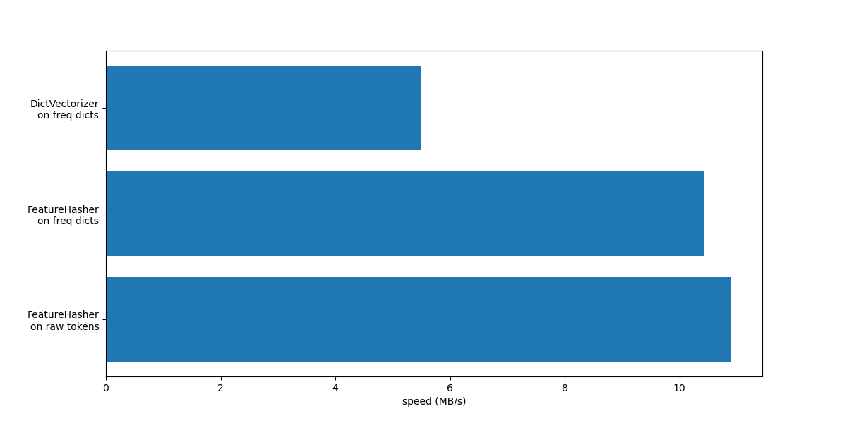
在这两种情况下,FeatureHasher 的速度大约是 DictVectorizer 的两倍。这在处理大量数据时非常方便,但缺点是失去了转换的可逆性,这反过来使得模型的解释成为一项更复杂的任务。
带有 input_type="string" 的 FeatureHeasher 略快于处理频率字典的变体,因为它不计算重复标记:每个标记被隐式计算一次,即使它被重复。根据下游的机器学习任务,这可能是一个限制,也可能不是。
与专用文本向量化器的比较#
CountVectorizer 接受原始数据,因为它在内部实现了标记化和出现次数计数。它与上一节中使用的带有自定义函数 token_freqs 的 DictVectorizer 相似。区别在于 CountVectorizer 更灵活。特别是,它通过 token_pattern 参数接受各种正则表达式模式。
from sklearn.feature_extraction.text import CountVectorizer

t0 = time()
vectorizer = CountVectorizer()
vectorizer.fit_transform(raw_data)
duration = time() - t0
dict_count_vectorizers["vectorizer"].append(vectorizer.__class__.__name__)
dict_count_vectorizers["speed"].append(data_size_mb / duration)
print(f"done in {duration:.3f} s at {data_size_mb / duration:.1f} MB/s")
print(f"Found {len(vectorizer.get_feature_names_out())} unique terms")
done in 0.570 s at 11.0 MB/s
Found 47885 unique terms
我们看到,使用 CountVectorizer 实现的速度大约是使用 DictVectorizer 以及我们定义的简单标记映射函数的两倍。原因是 CountVectorizer 通过对整个训练集重复使用已编译的正则表达式进行了优化,而不是像我们的简单标记化函数那样为每个文档创建一个正则表达式。
现在我们对 HashingVectorizer 进行类似的实验,它相当于结合了 FeatureHasher 类实现的“哈希技巧”和 CountVectorizer 的文本预处理和标记化。
from sklearn.feature_extraction.text import HashingVectorizer

t0 = time()
vectorizer = HashingVectorizer(n_features=2**18)
vectorizer.fit_transform(raw_data)
duration = time() - t0
dict_count_vectorizers["vectorizer"].append(vectorizer.__class__.__name__)
dict_count_vectorizers["speed"].append(data_size_mb / duration)
print(f"done in {duration:.3f} s at {data_size_mb / duration:.1f} MB/s")
done in 0.476 s at 13.1 MB/s
我们可以观察到,这是目前最快的文本标记化策略,前提是下游机器学习任务可以容忍少量冲突。
TfidfVectorizer#
在大型文本语料库中,某些词语出现频率较高(例如英语中的“the”、“a”、“is”),并且不携带有关文档实际内容的有意义信息。如果我们将词频数据直接提供给分类器,那些非常常见的术语将掩盖稀有但信息量更大的术语的频率。为了将计数特征重新加权为适合分类器使用的浮点值,通常使用 TfidfTransformer 实现的 tf-idf 转换。TF 代表“term-frequency”(词频),而“tf-idf”代表“term-frequency times inverse document-frequency”(词频乘以逆文档频率)。
我们现在对 TfidfVectorizer 进行基准测试,它相当于结合了 CountVectorizer 的标记化和出现次数计数以及 TfidfTransformer 的归一化和加权。
from sklearn.feature_extraction.text import TfidfVectorizer

t0 = time()
vectorizer = TfidfVectorizer()
vectorizer.fit_transform(raw_data)
duration = time() - t0
dict_count_vectorizers["vectorizer"].append(vectorizer.__class__.__name__)
dict_count_vectorizers["speed"].append(data_size_mb / duration)
print(f"done in {duration:.3f} s at {data_size_mb / duration:.1f} MB/s")
print(f"Found {len(vectorizer.get_feature_names_out())} unique terms")
done in 0.572 s at 10.9 MB/s
Found 47885 unique terms
总结#
让我们通过在单个图中总结所有记录的处理速度来结束本笔记本。
fig, ax = plt.subplots(figsize=(12, 6))

y_pos = np.arange(len(dict_count_vectorizers["vectorizer"]))
ax.barh(y_pos, dict_count_vectorizers["speed"], align="center")
ax.set_yticks(y_pos)
ax.set_yticklabels(dict_count_vectorizers["vectorizer"])
ax.invert_yaxis()
_ = ax.set_xlabel("speed (MB/s)")
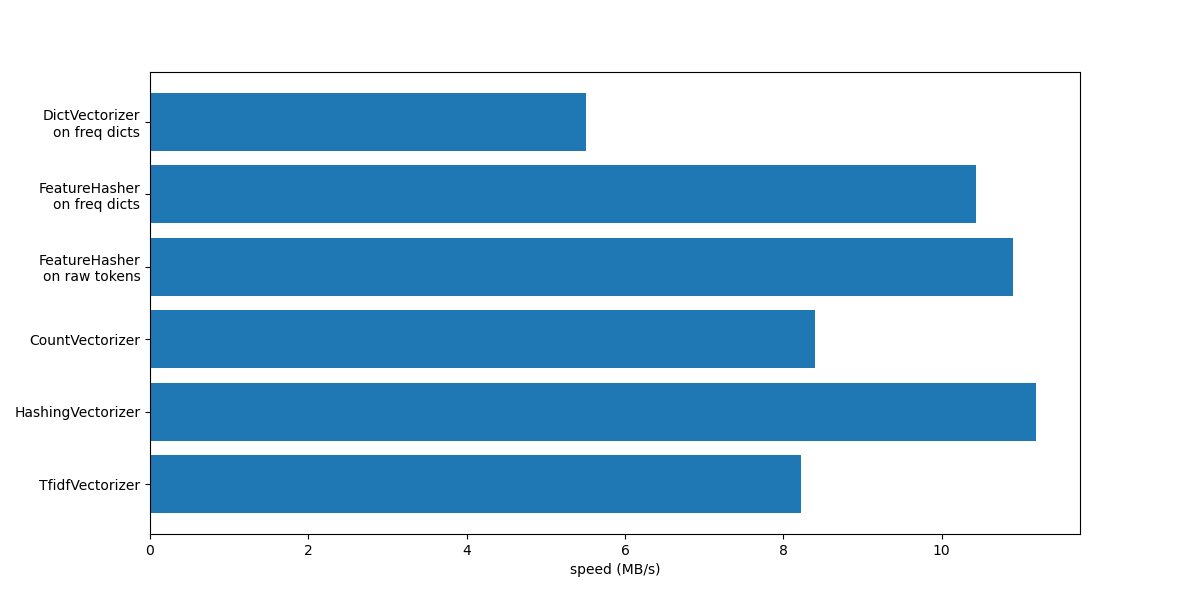
从图中可以看出,TfidfVectorizer 略慢于 CountVectorizer,因为 TfidfTransformer 引入了额外的操作。
另请注意,通过设置特征数 n_features = 2**18,HashingVectorizer 的性能优于 CountVectorizer,代价是由于哈希冲突导致转换不可逆。
我们强调 CountVectorizer 和 HashingVectorizer 在手动标记的文档上的性能优于等效的 DictVectorizer 和 FeatureHasher,因为前者向量化器的内部标记化步骤会编译一次正则表达式,然后将其重新用于所有文档。
脚本总运行时间: (0 minutes 4.607 seconds)
相关示例