注意
转到末尾 下载完整的示例代码或通过 JupyterLite 或 Binder 在浏览器中运行此示例。
基于模型和顺序特征选择#
此示例说明并比较了两种特征选择方法:基于特征重要性的 SelectFromModel,以及依赖贪婪方法的 SequentialFeatureSelector。
我们使用糖尿病数据集,该数据集包含从442名糖尿病患者收集的10个特征。
# Authors: The scikit-learn developers
# SPDX-License-Identifier: BSD-3-Clause
加载数据#
我们首先加载scikit-learn中可用的糖尿病数据集,并打印其描述
from sklearn.datasets import load_diabetes

diabetes = load_diabetes()
X, y = diabetes.data, diabetes.target
print(diabetes.DESCR)
.. _diabetes_dataset:

Diabetes dataset
----------------

Ten baseline variables, age, sex, body mass index, average blood
pressure, and six blood serum measurements were obtained for each of n =
442 diabetes patients, as well as the response of interest, a
quantitative measure of disease progression one year after baseline.

**Data Set Characteristics:**

:Number of Instances: 442

:Number of Attributes: First 10 columns are numeric predictive values

:Target: Column 11 is a quantitative measure of disease progression one year after baseline

:Attribute Information:
    - age     age in years
    - sex
    - bmi     body mass index
    - bp      average blood pressure
    - s1      tc, total serum cholesterol
    - s2      ldl, low-density lipoproteins
    - s3      hdl, high-density lipoproteins
    - s4      tch, total cholesterol / HDL
    - s5      ltg, possibly log of serum triglycerides level
    - s6      glu, blood sugar level

Note: Each of these 10 feature variables have been mean centered and scaled by the standard deviation times the square root of `n_samples` (i.e. the sum of squares of each column totals 1).

Source URL:
https://www4.stat.ncsu.edu/~boos/var.select/diabetes.html

For more information see:
Bradley Efron, Trevor Hastie, Iain Johnstone and Robert Tibshirani (2004) "Least Angle Regression," Annals of Statistics (with discussion), 407-499.
(https://web.stanford.edu/~hastie/Papers/LARS/LeastAngle_2002.pdf)
基于系数的特征重要性#
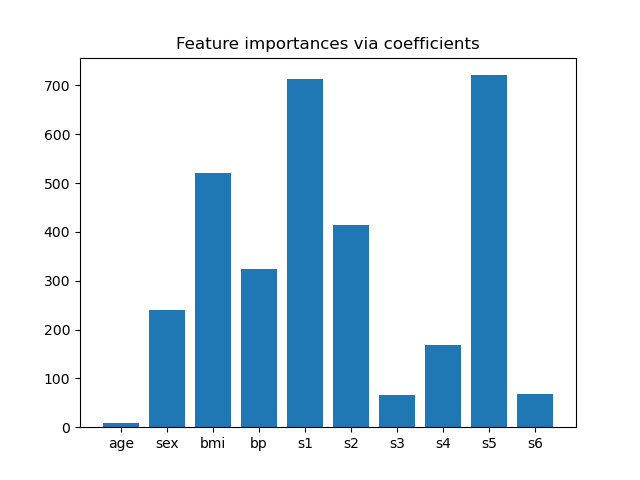
为了了解特征的重要性,我们将使用 RidgeCV 估计器。绝对 coef_ 值最高的特征被认为是最重要的。我们可以直接观察系数而无需对其进行缩放(或缩放数据),因为从上面的描述中我们知道特征已经标准化了。有关线性模型系数解释的更完整示例,您可以参考 线性模型系数解释中的常见陷阱。
import matplotlib.pyplot as plt
import numpy as np

from sklearn.linear_model import RidgeCV

ridge = RidgeCV(alphas=np.logspace(-6, 6, num=5)).fit(X, y)
importance = np.abs(ridge.coef_)
feature_names = np.array(diabetes.feature_names)
plt.bar(height=importance, x=feature_names)
plt.title("Feature importances via coefficients")
plt.show()

基于重要性选择特征#
现在我们想根据系数选择两个最重要的特征。SelectFromModel 正是为了这个目的。SelectFromModel 接受一个 threshold 参数,并将选择重要性(由系数定义)高于此阈值的特征。
由于我们只想选择2个特征,我们将把这个阈值设置得略高于第三个最重要特征的系数。
from time import time

from sklearn.feature_selection import SelectFromModel

threshold = np.sort(importance)[-3] + 0.01

tic = time()
sfm = SelectFromModel(ridge, threshold=threshold).fit(X, y)
toc = time()
print(f"Features selected by SelectFromModel: {feature_names[sfm.get_support()]}")
print(f"Done in {toc - tic:.3f}s")
Features selected by SelectFromModel: ['s1' 's5']
Done in 0.002s
使用顺序特征选择选择特征#
另一种选择特征的方法是使用 SequentialFeatureSelector (SFS)。SFS是一种贪婪过程,在每次迭代中,我们根据交叉验证分数选择要添加到已选特征集的最佳新特征。也就是说,我们从0个特征开始,选择分数最高的单个最佳特征。重复该过程,直到达到所需的选定特征数量。
我们也可以朝相反的方向进行(向后 SFS),即从所有特征开始,然后贪婪地逐个移除特征。我们在这里说明了这两种方法。
from sklearn.feature_selection import SequentialFeatureSelector

tic_fwd = time()
sfs_forward = SequentialFeatureSelector(
    ridge, n_features_to_select=2, direction="forward"
).fit(X, y)
toc_fwd = time()

tic_bwd = time()
sfs_backward = SequentialFeatureSelector(
    ridge, n_features_to_select=2, direction="backward"
).fit(X, y)
toc_bwd = time()

print(
    "Features selected by forward sequential selection: "
    f"{feature_names[sfs_forward.get_support()]}"
)
print(f"Done in {toc_fwd - tic_fwd:.3f}s")
print(
    "Features selected by backward sequential selection: "
    f"{feature_names[sfs_backward.get_support()]}"
)
print(f"Done in {toc_bwd - tic_bwd:.3f}s")
Features selected by forward sequential selection: ['bmi' 's5']
Done in 0.178s
Features selected by backward sequential selection: ['bmi' 's5']
Done in 0.515s
有趣的是,向前和向后选择选择了相同的特征集。一般来说,情况并非如此,两种方法会产生不同的结果。
我们还注意到SFS选择的特征与基于特征重要性选择的特征不同:SFS选择了 bmi 而不是 s1。这听起来相当合理,因为 bmi 对应于根据系数的第三个最重要的特征。考虑到SFS根本不使用系数,这非常值得注意。
最后,我们应该注意到 SelectFromModel 明显快于SFS。事实上,SelectFromModel 只需拟合一次模型,而SFS在每次迭代中都需要交叉验证许多不同的模型。然而,SFS适用于任何模型,而 SelectFromModel 要求底层估计器公开 coef_ 属性或 feature_importances_ 属性。向前SFS比向后SFS更快,因为它只需要执行 n_features_to_select = 2 次迭代,而向后SFS需要执行 n_features - n_features_to_select = 8 次迭代。
使用负容差值#
SequentialFeatureSelector 可用于移除数据集中存在的特征,并通过 direction="backward" 和 tol 的负值返回原始特征的一个较小子集。
我们首先加载乳腺癌数据集,该数据集包含30个不同的特征和569个样本。
import numpy as np

from sklearn.datasets import load_breast_cancer

breast_cancer_data = load_breast_cancer()
X, y = breast_cancer_data.data, breast_cancer_data.target
feature_names = np.array(breast_cancer_data.feature_names)
print(breast_cancer_data.DESCR)
.. _breast_cancer_dataset:

Breast cancer Wisconsin (diagnostic) dataset
--------------------------------------------

**Data Set Characteristics:**

:Number of Instances: 569

:Number of Attributes: 30 numeric, predictive attributes and the class

:Attribute Information:
    - radius (mean of distances from center to points on the perimeter)
    - texture (standard deviation of gray-scale values)
    - perimeter
    - area
    - smoothness (local variation in radius lengths)
    - compactness (perimeter^2 / area - 1.0)
    - concavity (severity of concave portions of the contour)
    - concave points (number of concave portions of the contour)
    - symmetry
    - fractal dimension ("coastline approximation" - 1)

    The mean, standard error, and "worst" or largest (mean of the three
    worst/largest values) of these features were computed for each image,
    resulting in 30 features.  For instance, field 0 is Mean Radius, field
    10 is Radius SE, field 20 is Worst Radius.

    - class:
            - WDBC-Malignant
            - WDBC-Benign

:Summary Statistics:

===================================== ====== ======
                                        Min    Max
===================================== ====== ======
radius (mean):                        6.981  28.11
texture (mean):                       9.71   39.28
perimeter (mean):                     43.79  188.5
area (mean):                          143.5  2501.0
smoothness (mean):                    0.053  0.163
compactness (mean):                   0.019  0.345
concavity (mean):                     0.0    0.427
concave points (mean):                0.0    0.201
symmetry (mean):                      0.106  0.304
fractal dimension (mean):             0.05   0.097
radius (standard error):              0.112  2.873
texture (standard error):             0.36   4.885
perimeter (standard error):           0.757  21.98
area (standard error):                6.802  542.2
smoothness (standard error):          0.002  0.031
compactness (standard error):         0.002  0.135
concavity (standard error):           0.0    0.396
concave points (standard error):      0.0    0.053
symmetry (standard error):            0.008  0.079
fractal dimension (standard error):   0.001  0.03
radius (worst):                       7.93   36.04
texture (worst):                      12.02  49.54
perimeter (worst):                    50.41  251.2
area (worst):                         185.2  4254.0
smoothness (worst):                   0.071  0.223
compactness (worst):                  0.027  1.058
concavity (worst):                    0.0    1.252
concave points (worst):               0.0    0.291
symmetry (worst):                     0.156  0.664
fractal dimension (worst):            0.055  0.208
===================================== ====== ======

:Missing Attribute Values: None

:Class Distribution: 212 - Malignant, 357 - Benign

:Creator:  Dr. William H. Wolberg, W. Nick Street, Olvi L. Mangasarian

:Donor: Nick Street

:Date: November, 1995

This is a copy of UCI ML Breast Cancer Wisconsin (Diagnostic) datasets.
https://goo.gl/U2Uwz2

Features are computed from a digitized image of a fine needle
aspirate (FNA) of a breast mass.  They describe
characteristics of the cell nuclei present in the image.

Separating plane described above was obtained using
Multisurface Method-Tree (MSM-T) [K. P. Bennett, "Decision Tree
Construction Via Linear Programming." Proceedings of the 4th
Midwest Artificial Intelligence and Cognitive Science Society,
pp. 97-101, 1992], a classification method which uses linear
programming to construct a decision tree.  Relevant features
were selected using an exhaustive search in the space of 1-4
features and 1-3 separating planes.

The actual linear program used to obtain the separating plane
in the 3-dimensional space is that described in:
[K. P. Bennett and O. L. Mangasarian: "Robust Linear
Programming Discrimination of Two Linearly Inseparable Sets",
Optimization Methods and Software 1, 1992, 23-34].

This database is also available through the UW CS ftp server:

ftp ftp.cs.wisc.edu
cd math-prog/cpo-dataset/machine-learn/WDBC/

.. dropdown:: References

  - W.N. Street, W.H. Wolberg and O.L. Mangasarian. Nuclear feature extraction
    for breast tumor diagnosis. IS&T/SPIE 1993 International Symposium on
    Electronic Imaging: Science and Technology, volume 1905, pages 861-870,
    San Jose, CA, 1993.
  - O.L. Mangasarian, W.N. Street and W.H. Wolberg. Breast cancer diagnosis and
    prognosis via linear programming. Operations Research, 43(4), pages 570-577,
    July-August 1995.
  - W.H. Wolberg, W.N. Street, and O.L. Mangasarian. Machine learning techniques
    to diagnose breast cancer from fine-needle aspirates. Cancer Letters 77 (1994)
    163-171.
我们将使用 LogisticRegression 估计器与 SequentialFeatureSelector 来执行特征选择。
from sklearn.linear_model import LogisticRegression
from sklearn.metrics import roc_auc_score
from sklearn.pipeline import make_pipeline
from sklearn.preprocessing import StandardScaler

for tol in [-1e-2, -1e-3, -1e-4]:
    start = time()
    feature_selector = SequentialFeatureSelector(
        LogisticRegression(),
        n_features_to_select="auto",
        direction="backward",
        scoring="roc_auc",
        tol=tol,
        n_jobs=2,
    )
    model = make_pipeline(StandardScaler(), feature_selector, LogisticRegression())
    model.fit(X, y)
    end = time()
    print(f"\ntol: {tol}")
    print(f"Features selected: {feature_names[model[1].get_support()]}")
    print(f"ROC AUC score: {roc_auc_score(y, model.predict_proba(X)[:, 1]):.3f}")
    print(f"Done in {end - start:.3f}s")
tol: -0.01
Features selected: ['worst perimeter']
ROC AUC score: 0.975
Done in 17.444s

tol: -0.001
Features selected: ['radius error' 'fractal dimension error' 'worst texture'
 'worst perimeter' 'worst concave points']
ROC AUC score: 0.997
Done in 17.263s

tol: -0.0001
Features selected: ['mean compactness' 'mean concavity' 'mean concave points' 'radius error'
 'area error' 'concave points error' 'symmetry error'
 'fractal dimension error' 'worst texture' 'worst perimeter' 'worst area'
 'worst concave points' 'worst symmetry']
ROC AUC score: 0.998
Done in 15.368s
我们可以看到,随着 tol 的负值接近零,选择的特征数量倾向于增加。随着 tol 的值接近零,特征选择所需的时间也会减少。
脚本总运行时间: (0 minutes 50.848 seconds)
相关示例


