DBSCAN 聚类算法演示

DBSCAN (Density-Based Spatial Clustering of Applications with Noise) 算法在高密度区域中寻找核心样本并从它们扩展聚类。此算法适用于包含类似密度聚类的数据。

有关 2D 数据集上不同聚类算法的演示，请参阅在玩具数据集上比较不同的聚类算法示例。

# Authors: The scikit-learn developers
# SPDX-License-Identifier: BSD-3-Clause

数据生成

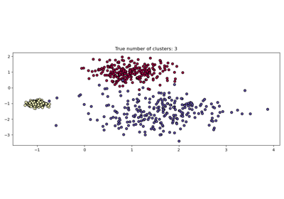
我们使用 make_blobs 创建 3 个合成聚类。

from sklearn.datasets import make_blobs
from sklearn.preprocessing import StandardScaler

centers = [[1, 1], [-1, -1], [1, -1]]
X, labels_true = make_blobs(
    n_samples=750, centers=centers, cluster_std=0.4, random_state=0
)

X = StandardScaler().fit_transform(X)

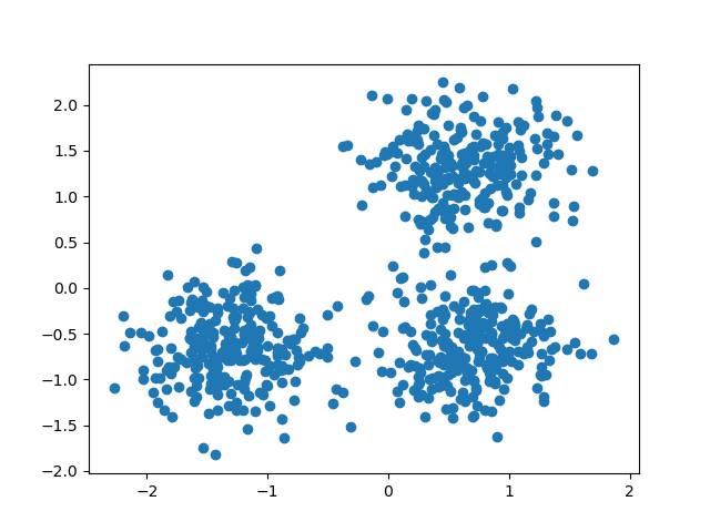
我们可以可视化生成的数据。

import matplotlib.pyplot as plt

plt.scatter(X[:, 0], X[:, 1])
plt.show()

计算 DBSCAN

可以使用 labels_ 属性访问 DBSCAN 分配的标签。噪声样本被赋予标签 \(-1\)。

import numpy as np

from sklearn import metrics
from sklearn.cluster import DBSCAN

db = DBSCAN(eps=0.3, min_samples=10).fit(X)
labels = db.labels_

# Number of clusters in labels, ignoring noise if present.
n_clusters_ = len(set(labels)) - (1 if -1 in labels else 0)
n_noise_ = list(labels).count(-1)

print("Estimated number of clusters: %d" % n_clusters_)
print("Estimated number of noise points: %d" % n_noise_)

Estimated number of clusters: 3
Estimated number of noise points: 18

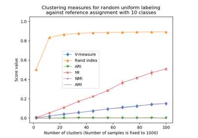
聚类算法本质上是无监督学习方法。然而，由于 make_blobs 提供了合成聚类的真实标签，因此可以使用利用这种“监督”真实信息的评估指标来量化结果聚类的质量。此类指标的示例包括同质性 (homogeneity)、完整性 (completeness)、V-measure、Rand-Index、Adjusted Rand-Index 和 Adjusted Mutual Information (AMI)。

如果真实标签未知，则只能使用模型结果本身进行评估。在这种情况下，轮廓系数 (Silhouette Coefficient) 会派上用场。

欲了解更多信息，请参阅聚类性能评估中的机会调整示例或聚类性能评估模块。

print(f"Homogeneity: {metrics.homogeneity_score(labels_true, labels):.3f}")
print(f"Completeness: {metrics.completeness_score(labels_true, labels):.3f}")
print(f"V-measure: {metrics.v_measure_score(labels_true, labels):.3f}")
print(f"Adjusted Rand Index: {metrics.adjusted_rand_score(labels_true, labels):.3f}")
print(
    "Adjusted Mutual Information:"
    f" {metrics.adjusted_mutual_info_score(labels_true, labels):.3f}"
)
print(f"Silhouette Coefficient: {metrics.silhouette_score(X, labels):.3f}")

Homogeneity: 0.953
Completeness: 0.883
V-measure: 0.917
Adjusted Rand Index: 0.952
Adjusted Mutual Information: 0.916
Silhouette Coefficient: 0.626

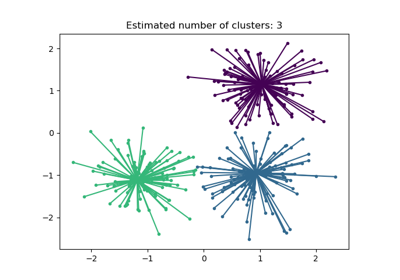
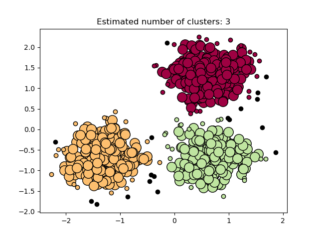
绘制结果

核心样本（大点）和非核心样本（小点）根据分配的聚类进行颜色编码。被标记为噪声的样本用黑色表示。

unique_labels = set(labels)
core_samples_mask = np.zeros_like(labels, dtype=bool)
core_samples_mask[db.core_sample_indices_] = True

colors = [plt.cm.Spectral(each) for each in np.linspace(0, 1, len(unique_labels))]
for k, col in zip(unique_labels, colors):
    if k == -1:
        # Black used for noise.
        col = [0, 0, 0, 1]

    class_member_mask = labels == k

    xy = X[class_member_mask & core_samples_mask]
    plt.plot(
        xy[:, 0],
        xy[:, 1],
        "o",
        markerfacecolor=tuple(col),
        markeredgecolor="k",
        markersize=14,
    )

    xy = X[class_member_mask & ~core_samples_mask]
    plt.plot(
        xy[:, 0],
        xy[:, 1],
        "o",
        markerfacecolor=tuple(col),
        markeredgecolor="k",
        markersize=6,
    )

plt.title(f"Estimated number of clusters: {n_clusters_}")
plt.show()

相关示例

亲和传播聚类算法演示

亲和传播聚类算法演示

聚类性能评估中的机会调整

聚类性能评估中的机会调整

HDBSCAN 聚类算法演示

HDBSCAN 聚类算法演示

均值漂移聚类算法演示

均值漂移聚类算法演示