注意
转到末尾 下载完整示例代码。或通过 JupyterLite 或 Binder 在浏览器中运行此示例
梯度提升回归的预测区间#
本示例展示了如何使用分位数回归创建预测区间。有关 HistGradientBoostingRegressor 的其他一些功能示例,请参阅 直方图梯度提升树中的特征。
# Authors: The scikit-learn developers
# SPDX-License-Identifier: BSD-3-Clause
通过将函数 f 应用于均匀采样的随机输入,生成一个合成回归问题的数据。
import numpy as np

from sklearn.model_selection import train_test_split


def f(x):
    """The function to predict."""
    return x * np.sin(x)


rng = np.random.RandomState(42)
X = np.atleast_2d(rng.uniform(0, 10.0, size=1000)).T
expected_y = f(X).ravel()
为了使问题更有趣,我们将目标 y 的观测值生成为由函数 f 计算的确定项和服从中心对数正态分布的随机噪声项之和。为了使其更加有趣,我们考虑噪声幅度取决于输入变量 x(异方差噪声)的情况。
对数正态分布是非对称且长尾的:观测到大异常值是可能的,但不可能观测到小异常值。
sigma = 0.5 + X.ravel() / 10
noise = rng.lognormal(sigma=sigma) - np.exp(sigma**2 / 2)
y = expected_y + noise
分割成训练集和测试集
X_train, X_test, y_train, y_test = train_test_split(X, y, random_state=0)
拟合非线性分位数和最小二乘回归器#
拟合使用分位数损失和 alpha=0.05, 0.5, 0.95 训练的梯度提升模型。
为 alpha=0.05 和 alpha=0.95 获得的模型会产生一个 90% 的置信区间(95% - 5% = 90%)。
使用 alpha=0.5 训练的模型会产生一个中位数回归:平均而言,目标观测值在预测值之上和之下应该数量相同。
from sklearn.ensemble import GradientBoostingRegressor
from sklearn.metrics import mean_pinball_loss, mean_squared_error

all_models = {}
common_params = dict(
    learning_rate=0.05,
    n_estimators=200,
    max_depth=2,
    min_samples_leaf=9,
    min_samples_split=9,
)
for alpha in [0.05, 0.5, 0.95]:
    gbr = GradientBoostingRegressor(loss="quantile", alpha=alpha, **common_params)
    all_models["q %1.2f" % alpha] = gbr.fit(X_train, y_train)
请注意,从中间数据集(n_samples >= 10_000)开始,HistGradientBoostingRegressor 比 GradientBoostingRegressor 快得多,本示例并非如此。
为了比较,我们还拟合了一个使用常用(均方)误差(MSE)训练的基线模型。
gbr_ls = GradientBoostingRegressor(loss="squared_error", **common_params)
all_models["mse"] = gbr_ls.fit(X_train, y_train)
创建一个范围为 [0, 10] 的均匀间隔输入值评估集。
xx = np.atleast_2d(np.linspace(0, 10, 1000)).T
绘制真实的条件均值函数 f、条件均值预测(损失等于平方误差)、条件中位数和条件 90% 区间(从第 5 到第 95 条件百分位数)。
import matplotlib.pyplot as plt

y_pred = all_models["mse"].predict(xx)
y_lower = all_models["q 0.05"].predict(xx)
y_upper = all_models["q 0.95"].predict(xx)
y_med = all_models["q 0.50"].predict(xx)

fig = plt.figure(figsize=(10, 10))
plt.plot(xx, f(xx), "black", linewidth=3, label=r"$f(x) = x\,\sin(x)$")
plt.plot(X_test, y_test, "b.", markersize=10, label="Test observations")
plt.plot(xx, y_med, "tab:orange", linewidth=3, label="Predicted median")
plt.plot(xx, y_pred, "tab:green", linewidth=3, label="Predicted mean")
plt.fill_between(
    xx.ravel(), y_lower, y_upper, alpha=0.4, label="Predicted 90% interval"
)
plt.xlabel("$x$")
plt.ylabel("$f(x)$")
plt.ylim(-10, 25)
plt.legend(loc="upper left")
plt.show()
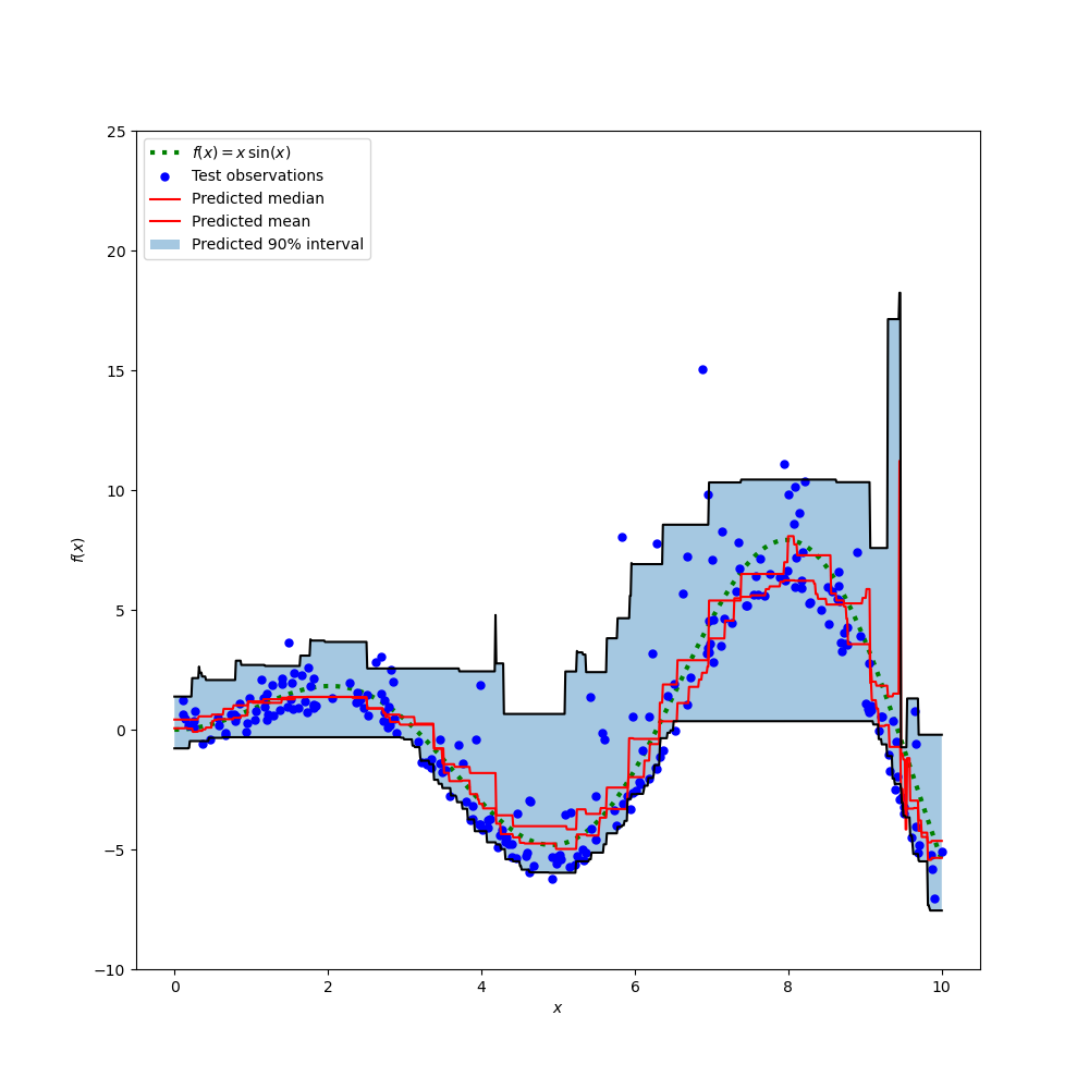
比较预测中位数和预测均值,我们注意到中位数平均低于均值,因为噪声偏向于高值(大异常值)。中位数估计也似乎更平滑,因为它对异常值具有天然的鲁棒性。
此外,我们还观察到,梯度提升树的归纳偏差不幸地阻止了我们的 0.05 分位数完全捕捉信号的正弦形状,尤其是在 x=8 附近。调整超参数可以减少这种影响,如本笔记本的最后一部分所示。
误差指标分析#
在训练数据集上使用 mean_squared_error 和 mean_pinball_loss 指标评估模型。
import pandas as pd


def highlight_min(x):
    x_min = x.min()
    return ["font-weight: bold" if v == x_min else "" for v in x]


results = []
for name, gbr in sorted(all_models.items()):
    metrics = {"model": name}
    y_pred = gbr.predict(X_train)
    for alpha in [0.05, 0.5, 0.95]:
        metrics["pbl=%1.2f" % alpha] = mean_pinball_loss(y_train, y_pred, alpha=alpha)
    metrics["MSE"] = mean_squared_error(y_train, y_pred)
    results.append(metrics)

pd.DataFrame(results).set_index("model").style.apply(highlight_min)
一列显示所有使用相同指标评估的模型。当模型使用相同指标进行训练和衡量时,该列应获得最小值。如果训练收敛,在训练集上始终应该如此。
请注意,由于目标分布是非对称的,预期条件均值和条件中位数显著不同,因此不能使用平方误差模型来很好地估计条件中位数,反之亦然。
如果目标分布是对称的且没有异常值(例如,带有高斯噪声),那么中位数估计器和最小二乘估计器将产生相似的预测。
然后我们在测试集上执行相同的操作。
results = []
for name, gbr in sorted(all_models.items()):
    metrics = {"model": name}
    y_pred = gbr.predict(X_test)
    for alpha in [0.05, 0.5, 0.95]:
        metrics["pbl=%1.2f" % alpha] = mean_pinball_loss(y_test, y_pred, alpha=alpha)
    metrics["MSE"] = mean_squared_error(y_test, y_pred)
    results.append(metrics)

pd.DataFrame(results).set_index("model").style.apply(highlight_min)
误差更高,意味着模型略微过拟合了数据。这仍然表明,当模型通过最小化相同的指标进行训练时,可以获得最佳测试指标。
请注意,条件中位数估计器在测试集上的 MSE 方面与平方误差估计器具有竞争力:这可以通过平方误差估计器对大异常值非常敏感并可能导致显著过拟合的事实来解释。这可以在上一张图的右侧看到。条件中位数估计器存在偏差(对于这种非对称噪声是低估),但它对异常值也具有天然的鲁棒性,并且过拟合较少。
置信区间的校准#
我们还可以评估两个极端分位数估计器生成良好校准的条件 90% 置信区间的能力。
为此,我们可以计算落在预测之间的观测值比例
def coverage_fraction(y, y_low, y_high):
    return np.mean(np.logical_and(y >= y_low, y <= y_high))


coverage_fraction(
    y_train,
    all_models["q 0.05"].predict(X_train),
    all_models["q 0.95"].predict(X_train),
)
np.float64(0.9)
在训练集上,校准值非常接近 90% 置信区间的预期覆盖值。
coverage_fraction(
    y_test, all_models["q 0.05"].predict(X_test), all_models["q 0.95"].predict(X_test)
)
np.float64(0.868)
在测试集上,估计的置信区间略窄。但请注意,我们需要将这些指标包装在交叉验证循环中,以评估它们在数据重采样下的变异性。
调优分位数回归器的超参数#
在上图中,我们观察到第 5 百分位数回归器似乎欠拟合,并且无法适应信号的正弦形状。
模型的超参数是为中位数回归器手动大致调优的,没有理由认为相同的超参数适用于第 5 百分位数回归器。
为了证实这一假设,我们通过在 alpha=0.05 的弹珠损失上进行交叉验证来选择最佳模型参数,从而调优一个新的第 5 百分位数回归器的超参数。
from pprint import pprint

from sklearn.experimental import enable_halving_search_cv  # noqa: F401
from sklearn.metrics import make_scorer
from sklearn.model_selection import HalvingRandomSearchCV

param_grid = dict(
    learning_rate=[0.05, 0.1, 0.2],
    max_depth=[2, 5, 10],
    min_samples_leaf=[1, 5, 10, 20],
    min_samples_split=[5, 10, 20, 30, 50],
)
alpha = 0.05
neg_mean_pinball_loss_05p_scorer = make_scorer(
    mean_pinball_loss,
    alpha=alpha,
    greater_is_better=False,  # maximize the negative loss
)
gbr = GradientBoostingRegressor(loss="quantile", alpha=alpha, random_state=0)
search_05p = HalvingRandomSearchCV(
    gbr,
    param_grid,
    resource="n_estimators",
    max_resources=250,
    min_resources=50,
    scoring=neg_mean_pinball_loss_05p_scorer,
    n_jobs=2,
    random_state=0,
).fit(X_train, y_train)
pprint(search_05p.best_params_)
{'learning_rate': 0.2,
 'max_depth': 2,
 'min_samples_leaf': 20,
 'min_samples_split': 10,
 'n_estimators': 150}
我们观察到,为中位数回归器手动调优的超参数与适合第 5 百分位数回归器的超参数在同一范围内。
现在让我们为第 95 百分位数回归器调优超参数。我们需要重新定义用于选择最佳模型的 scoring 指标,并调整内部梯度提升估计器本身的 alpha 参数。
from sklearn.base import clone

alpha = 0.95
neg_mean_pinball_loss_95p_scorer = make_scorer(
    mean_pinball_loss,
    alpha=alpha,
    greater_is_better=False,  # maximize the negative loss
)
search_95p = clone(search_05p).set_params(
    estimator__alpha=alpha,
    scoring=neg_mean_pinball_loss_95p_scorer,
)
search_95p.fit(X_train, y_train)
pprint(search_95p.best_params_)
{'learning_rate': 0.05,
 'max_depth': 2,
 'min_samples_leaf': 5,
 'min_samples_split': 20,
 'n_estimators': 150}
结果显示,搜索过程为第 95 百分位数回归器识别的超参数大致与为中位数回归器手动调优的超参数以及为第 5 百分位数回归器通过搜索过程识别的超参数在同一范围内。然而,超参数搜索确实导致了改进的 90% 置信区间,该区间由这两个调优后的分位数回归器的预测构成。请注意,由于异常值的存在,上 95 百分位数的预测形状比下 5 百分位数的预测形状粗糙得多。
y_lower = search_05p.predict(xx)
y_upper = search_95p.predict(xx)

fig = plt.figure(figsize=(10, 10))
plt.plot(xx, f(xx), "black", linewidth=3, label=r"$f(x) = x\,\sin(x)$")
plt.plot(X_test, y_test, "b.", markersize=10, label="Test observations")
plt.fill_between(
    xx.ravel(), y_lower, y_upper, alpha=0.4, label="Predicted 90% interval"
)
plt.xlabel("$x$")
plt.ylabel("$f(x)$")
plt.ylim(-10, 25)
plt.legend(loc="upper left")
plt.title("Prediction with tuned hyper-parameters")
plt.show()
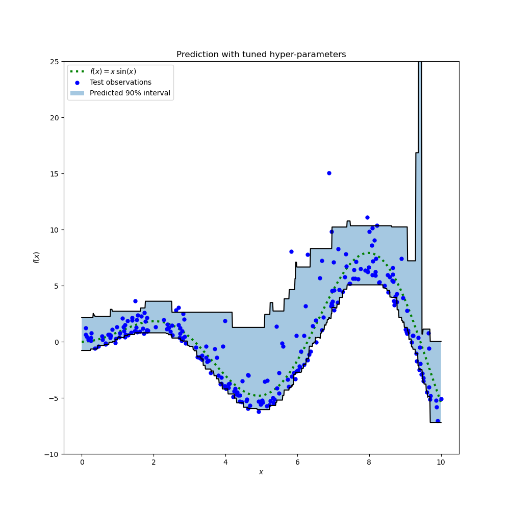
该图在质量上看起来比未调优的模型更好,尤其是在较低分位数的形状方面。
现在我们定量评估这对估计器的联合校准
coverage_fraction(y_train, search_05p.predict(X_train), search_95p.predict(X_train))
np.float64(0.9026666666666666)
coverage_fraction(y_test, search_05p.predict(X_test), search_95p.predict(X_test))
np.float64(0.796)
调优后的这对估计器在测试集上的校准效果不幸地没有更好:估计的置信区间宽度仍然太窄。
再次,我们需要将这项研究包装在交叉验证循环中,以更好地评估这些估计的变异性。
脚本总运行时间: (0 分钟 10.113 秒)


相关示例