注意
跳转到底部 下载完整示例代码。或者通过 JupyterLite 或 Binder 在浏览器中运行此示例
使用轮廓分析在KMeans聚类中选择聚类数量#
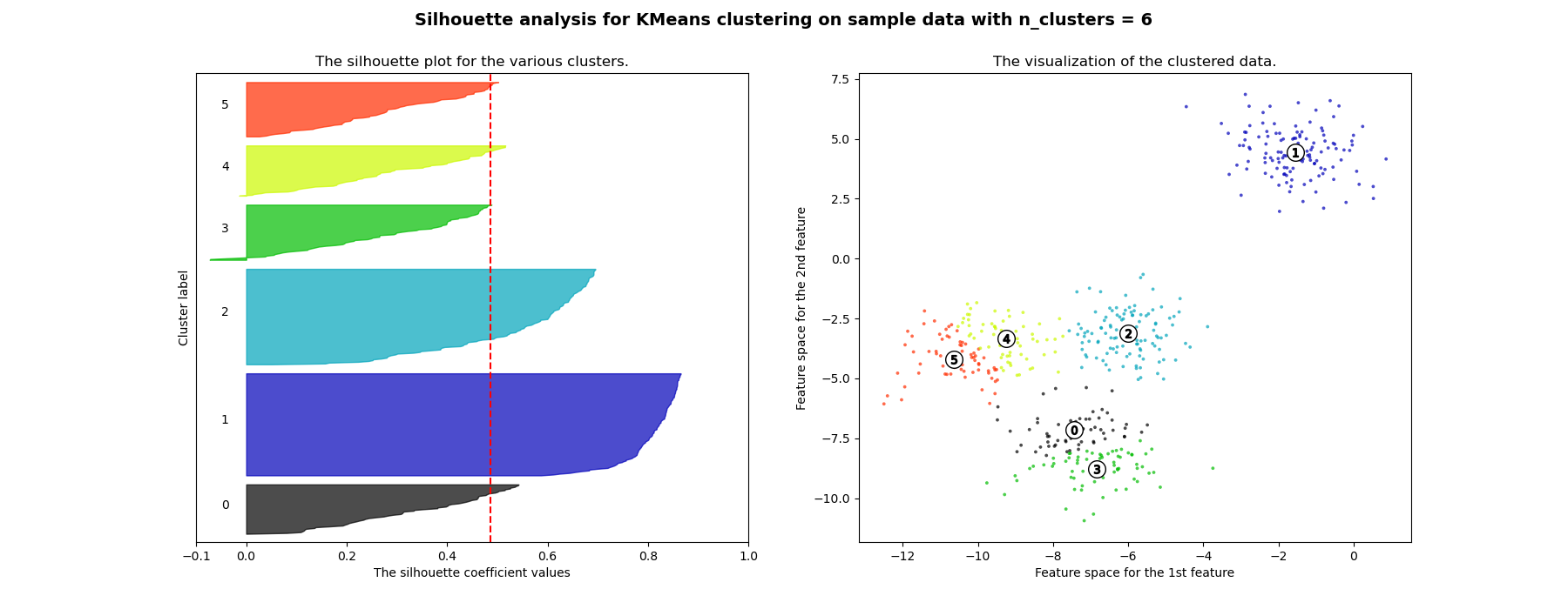
轮廓分析可用于研究生成聚类之间的分离距离。轮廓图显示了每个聚类中的点与其相邻聚类中的点之间的接近程度,从而提供了一种直观评估聚类数量等参数的方法。该度量值的范围是 [-1, 1]。
轮廓系数(这些值被称为)接近 +1 表明样本远离相邻聚类。值为 0 表示样本位于或非常接近两个相邻聚类之间的决策边界,负值表示这些样本可能已被分配到错误的聚类。
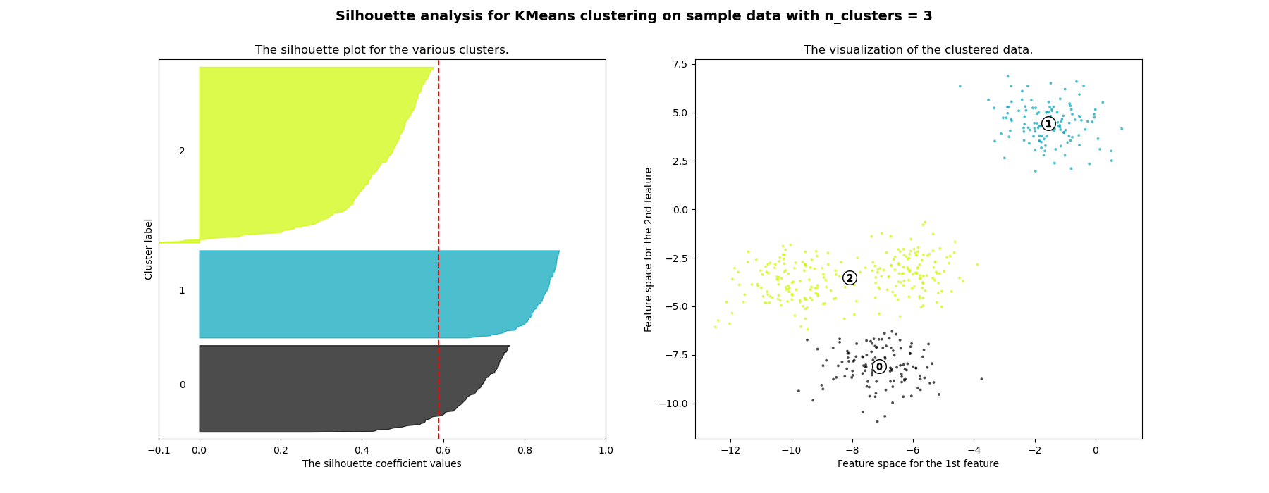
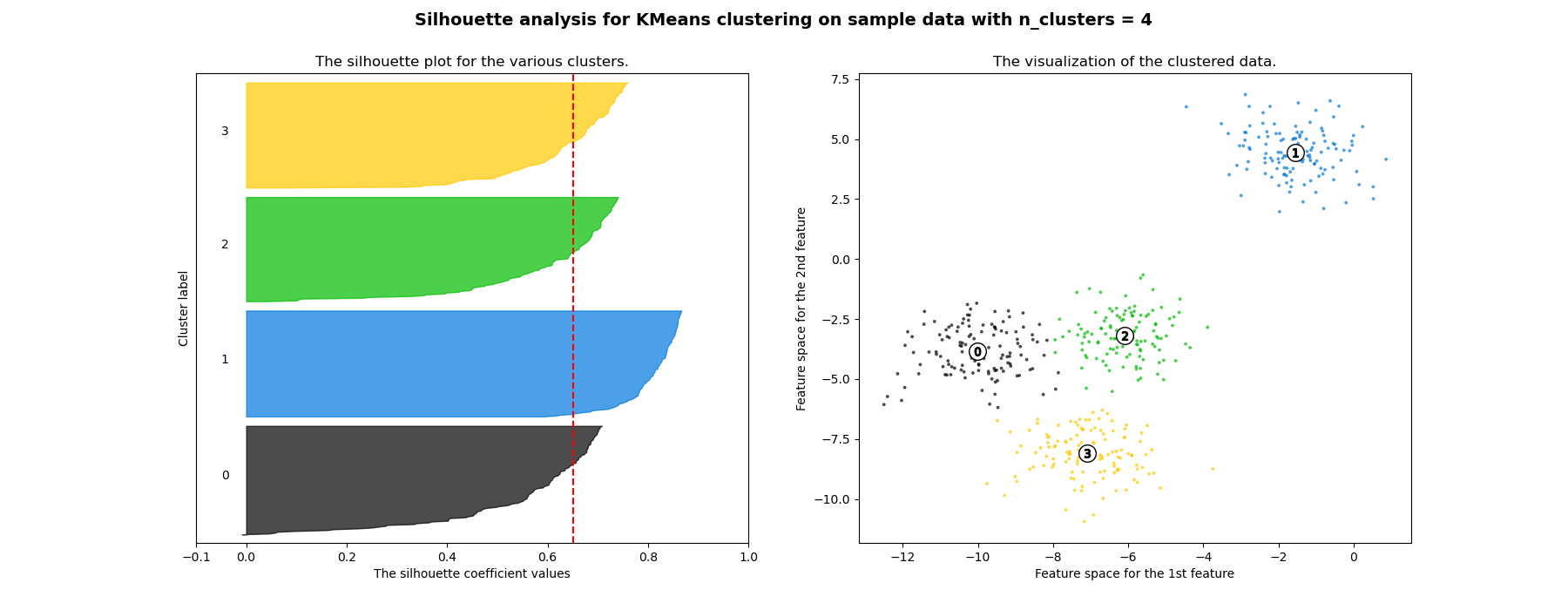
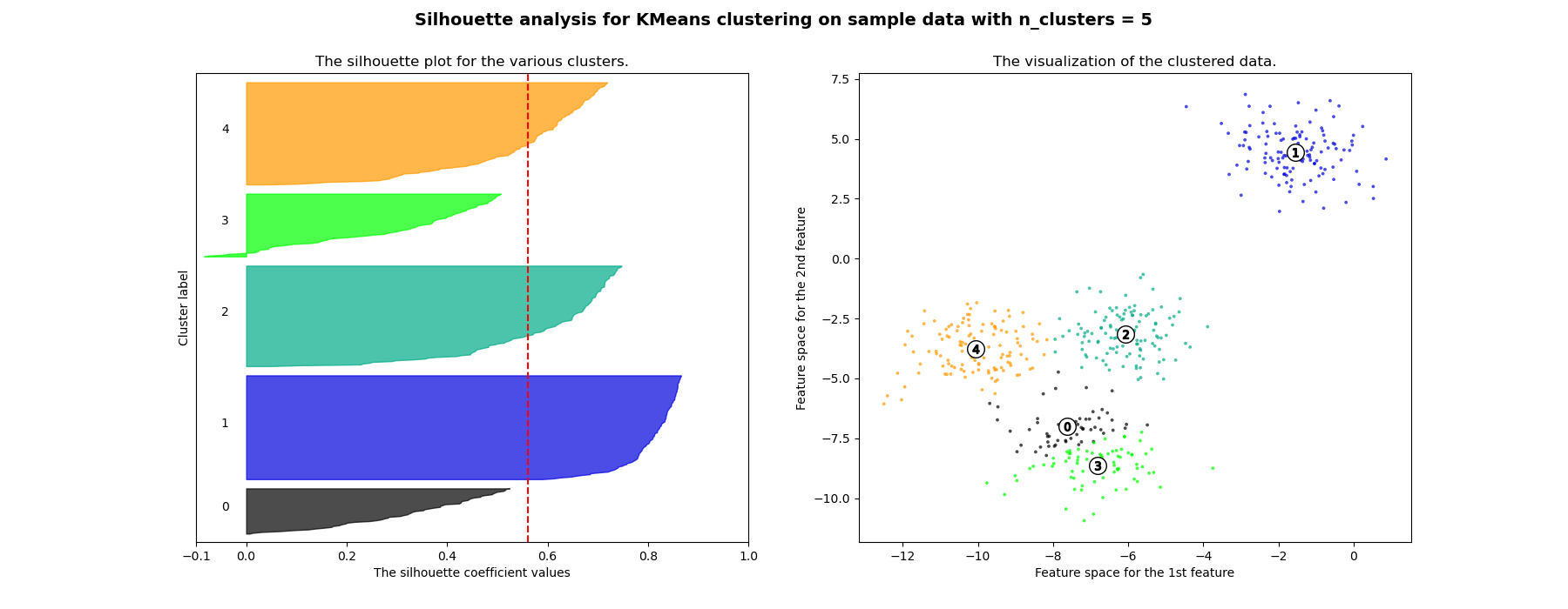
在此示例中,轮廓分析用于选择 n_clusters 的最优值。轮廓图显示,对于给定数据,n_clusters 的值选择 3、5 和 6 并不理想,这是因为存在轮廓分数低于平均水平的聚类,并且轮廓图的大小波动较大。轮廓分析在选择 2 和 4 之间时更为模糊。
此外,从轮廓图的厚度也可以可视化聚类大小。当 n_clusters 等于 2 时,聚类 0 的轮廓图由于将 3 个子聚类分组为一个大聚类而尺寸更大。然而,当 n_clusters 等于 4 时,所有图的厚度或多或少相似,因此大小也相似,这也可以从右侧的带标签散点图中得到验证。
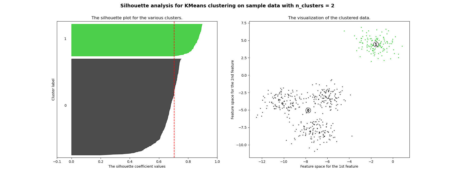
For n_clusters = 2 The average silhouette_score is : 0.7049787496083262
For n_clusters = 3 The average silhouette_score is : 0.5882004012129721
For n_clusters = 4 The average silhouette_score is : 0.6505186632729437
For n_clusters = 5 The average silhouette_score is : 0.561464362648773
For n_clusters = 6 The average silhouette_score is : 0.4857596147013469
# Authors: The scikit-learn developers
# SPDX-License-Identifier: BSD-3-Clause

import matplotlib.cm as cm
import matplotlib.pyplot as plt
import numpy as np

from sklearn.cluster import KMeans
from sklearn.datasets import make_blobs
from sklearn.metrics import silhouette_samples, silhouette_score

# Generating the sample data from make_blobs
# This particular setting has one distinct cluster and 3 clusters placed close
# together.
X, y = make_blobs(
    n_samples=500,
    n_features=2,
    centers=4,
    cluster_std=1,
    center_box=(-10.0, 10.0),
    shuffle=True,
    random_state=1,
)  # For reproducibility

range_n_clusters = [2, 3, 4, 5, 6]

for n_clusters in range_n_clusters:
    # Create a subplot with 1 row and 2 columns
    fig, (ax1, ax2) = plt.subplots(1, 2)
    fig.set_size_inches(18, 7)

    # The 1st subplot is the silhouette plot
    # The silhouette coefficient can range from -1, 1 but in this example all
    # lie within [-0.1, 1]
    ax1.set_xlim([-0.1, 1])
    # The (n_clusters+1)*10 is for inserting blank space between silhouette
    # plots of individual clusters, to demarcate them clearly.
    ax1.set_ylim([0, len(X) + (n_clusters + 1) * 10])

    # Initialize the clusterer with n_clusters value and a random generator
    # seed of 10 for reproducibility.
    clusterer = KMeans(n_clusters=n_clusters, random_state=10)
    cluster_labels = clusterer.fit_predict(X)

    # The silhouette_score gives the average value for all the samples.
    # This gives a perspective into the density and separation of the formed
    # clusters
    silhouette_avg = silhouette_score(X, cluster_labels)
    print(
        "For n_clusters =",
        n_clusters,
        "The average silhouette_score is :",
        silhouette_avg,
    )

    # Compute the silhouette scores for each sample
    sample_silhouette_values = silhouette_samples(X, cluster_labels)

    y_lower = 10
    for i in range(n_clusters):
        # Aggregate the silhouette scores for samples belonging to
        # cluster i, and sort them
        ith_cluster_silhouette_values = sample_silhouette_values[cluster_labels == i]

        ith_cluster_silhouette_values.sort()

        size_cluster_i = ith_cluster_silhouette_values.shape[0]
        y_upper = y_lower + size_cluster_i

        color = cm.nipy_spectral(float(i) / n_clusters)
        ax1.fill_betweenx(
            np.arange(y_lower, y_upper),
            0,
            ith_cluster_silhouette_values,
            facecolor=color,
            edgecolor=color,
            alpha=0.7,
        )

        # Label the silhouette plots with their cluster numbers at the middle
        ax1.text(-0.05, y_lower + 0.5 * size_cluster_i, str(i))

        # Compute the new y_lower for next plot
        y_lower = y_upper + 10  # 10 for the 0 samples

    ax1.set_title("The silhouette plot for the various clusters.")
    ax1.set_xlabel("The silhouette coefficient values")
    ax1.set_ylabel("Cluster label")

    # The vertical line for average silhouette score of all the values
    ax1.axvline(x=silhouette_avg, color="red", linestyle="--")

    ax1.set_yticks([])  # Clear the yaxis labels / ticks
    ax1.set_xticks([-0.1, 0, 0.2, 0.4, 0.6, 0.8, 1])

    # 2nd Plot showing the actual clusters formed
    colors = cm.nipy_spectral(cluster_labels.astype(float) / n_clusters)
    ax2.scatter(
        X[:, 0], X[:, 1], marker=".", s=30, lw=0, alpha=0.7, c=colors, edgecolor="k"
    )

    # Labeling the clusters
    centers = clusterer.cluster_centers_
    # Draw white circles at cluster centers
    ax2.scatter(
        centers[:, 0],
        centers[:, 1],
        marker="o",
        c="white",
        alpha=1,
        s=200,
        edgecolor="k",
    )

    for i, c in enumerate(centers):
        ax2.scatter(c[0], c[1], marker="$%d$" % i, alpha=1, s=50, edgecolor="k")

    ax2.set_title("The visualization of the clustered data.")
    ax2.set_xlabel("Feature space for the 1st feature")
    ax2.set_ylabel("Feature space for the 2nd feature")

    plt.suptitle(
        "Silhouette analysis for KMeans clustering on sample data with n_clusters = %d"
        % n_clusters,
        fontsize=14,
        fontweight="bold",
    )

plt.show()
脚本总运行时间:(0 分钟 1.067 秒)


相关示例