注意
跳到末尾 下载完整示例代码。或通过 JupyterLite 或 Binder 在浏览器中运行此示例
层次聚类:结构化与非结构化 Ward#
本示例构建了一个瑞士卷数据集,并对其位置运行层次聚类。
更多信息,请参阅 层次聚类。
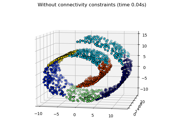
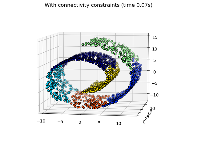
第一步,层次聚类在结构上不施加连通性约束,仅基于距离进行;第二步,聚类被限制在 k-最近邻图上:这是一种具有结构先验的层次聚类。
在没有连通性约束的情况下学习的一些簇不符合瑞士卷的结构,并跨越流形的不同折叠。相反,在施加连通性约束时,簇形成了瑞士卷的良好分区。
# Authors: The scikit-learn developers
# SPDX-License-Identifier: BSD-3-Clause

import time as time

# The following import is required
# for 3D projection to work with matplotlib < 3.2
import mpl_toolkits.mplot3d  # noqa: F401
import numpy as np
生成数据#
我们首先生成瑞士卷数据集。
from sklearn.datasets import make_swiss_roll

n_samples = 1500
noise = 0.05
X, _ = make_swiss_roll(n_samples, noise=noise)
# Make it thinner
X[:, 1] *= 0.5
计算聚类#
我们执行 AgglomerativeClustering(属于层次聚类),不施加任何连通性约束。
from sklearn.cluster import AgglomerativeClustering

print("Compute unstructured hierarchical clustering...")
st = time.time()
ward = AgglomerativeClustering(n_clusters=6, linkage="ward").fit(X)
elapsed_time = time.time() - st
label = ward.labels_
print(f"Elapsed time: {elapsed_time:.2f}s")
print(f"Number of points: {label.size}")
Compute unstructured hierarchical clustering...
Elapsed time: 0.03s
Number of points: 1500
绘制结果#
绘制非结构化层次聚类。
import matplotlib.pyplot as plt

fig1 = plt.figure()
ax1 = fig1.add_subplot(111, projection="3d", elev=7, azim=-80)
ax1.set_position([0, 0, 0.95, 1])
for l in np.unique(label):
    ax1.scatter(
        X[label == l, 0],
        X[label == l, 1],
        X[label == l, 2],
        color=plt.cm.jet(float(l) / np.max(label + 1)),
        s=20,
        edgecolor="k",
    )
_ = fig1.suptitle(f"Without connectivity constraints (time {elapsed_time:.2f}s)")
我们定义 k-最近邻,邻居数为 10#
from sklearn.neighbors import kneighbors_graph

connectivity = kneighbors_graph(X, n_neighbors=10, include_self=False)
计算聚类#
我们再次执行 AgglomerativeClustering,施加连通性约束。
print("Compute structured hierarchical clustering...")
st = time.time()
ward = AgglomerativeClustering(
    n_clusters=6, connectivity=connectivity, linkage="ward"
).fit(X)
elapsed_time = time.time() - st
label = ward.labels_
print(f"Elapsed time: {elapsed_time:.2f}s")
print(f"Number of points: {label.size}")
Compute structured hierarchical clustering...
Elapsed time: 0.06s
Number of points: 1500
绘制结果#
绘制结构化层次聚类。
fig2 = plt.figure()
ax2 = fig2.add_subplot(121, projection="3d", elev=7, azim=-80)
ax2.set_position([0, 0, 0.95, 1])
for l in np.unique(label):
    ax2.scatter(
        X[label == l, 0],
        X[label == l, 1],
        X[label == l, 2],
        color=plt.cm.jet(float(l) / np.max(label + 1)),
        s=20,
        edgecolor="k",
    )
fig2.suptitle(f"With connectivity constraints (time {elapsed_time:.2f}s)")

plt.show()
脚本总运行时间: (0 分钟 0.378 秒)


相关示例