注意
转到末尾以下载完整示例代码或通过JupyterLite或Binder在浏览器中运行此示例。
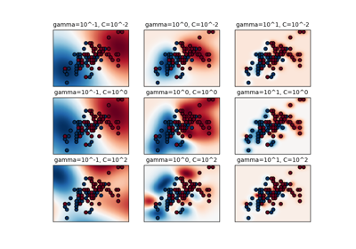
使用不同的SVM核函数绘制分类边界#
此示例展示了在二元、二维分类问题中,SVC(支持向量分类器)中的不同核函数如何影响分类边界。
SVC旨在通过最大化每类最外层数据点之间的边距,找到一个能有效分离训练数据中类别的超平面。这是通过找到最佳权重向量\(w\)来实现的,该向量定义了决策边界超平面,并最小化由hinge_loss函数测量的错误分类样本的合页损失之和。默认情况下,应用正则化参数C=1,这允许一定程度的误分类容忍度。
如果数据在原始特征空间中不是线性可分的,可以设置非线性核参数。根据核函数的不同,这个过程涉及添加新特征或转换现有特征,以丰富并可能增加数据的意义。当设置非"linear"的核函数时,SVC会应用核技巧(kernel trick),它使用核函数计算数据点对之间的相似性,而无需显式转换整个数据集。核技巧通过只考虑所有数据点对之间的关系,超越了原本必需的整个数据集的矩阵转换。核函数使用点积将两个向量(每对观测值)映射到它们的相似性。
然后可以使用核函数来计算超平面,就像数据集表示在更高维空间中一样。使用核函数而不是显式矩阵转换可以提高性能,因为核函数的时间复杂度为\(O({n}^2)\),而矩阵转换的复杂度取决于应用的具体转换。
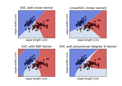
在此示例中,我们比较了支持向量机中最常见的核类型:线性核("linear")、多项式核("poly")、径向基函数核("rbf")和S形核("sigmoid")。
# Authors: The scikit-learn developers
# SPDX-License-Identifier: BSD-3-Clause
创建数据集#
我们创建一个包含16个样本和两个类别的二维分类数据集。我们绘制样本,颜色与各自的目标匹配。
import matplotlib.pyplot as plt
import numpy as np

X = np.array(
    [
        [0.4, -0.7],
        [-1.5, -1.0],
        [-1.4, -0.9],
        [-1.3, -1.2],
        [-1.1, -0.2],
        [-1.2, -0.4],
        [-0.5, 1.2],
        [-1.5, 2.1],
        [1.0, 1.0],
        [1.3, 0.8],
        [1.2, 0.5],
        [0.2, -2.0],
        [0.5, -2.4],
        [0.2, -2.3],
        [0.0, -2.7],
        [1.3, 2.1],
    ]
)

y = np.array([0, 0, 0, 0, 0, 0, 0, 0, 1, 1, 1, 1, 1, 1, 1, 1])

# Plotting settings
fig, ax = plt.subplots(figsize=(4, 3))
x_min, x_max, y_min, y_max = -3, 3, -3, 3
ax.set(xlim=(x_min, x_max), ylim=(y_min, y_max))

# Plot samples by color and add legend
scatter = ax.scatter(X[:, 0], X[:, 1], s=150, c=y, label=y, edgecolors="k")
ax.legend(*scatter.legend_elements(), loc="upper right", title="Classes")
ax.set_title("Samples in two-dimensional feature space")
plt.show()
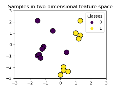
我们可以看到样本不能被一条直线清晰地分离。
训练SVC模型并绘制决策边界#
我们定义一个函数,该函数拟合一个SVC分类器,允许将kernel参数作为输入,然后使用DecisionBoundaryDisplay绘制模型学习到的决策边界。
请注意,为了简单起见,在此示例中,C参数设置为其默认值(C=1),gamma参数设置为gamma=2适用于所有核函数,尽管对于线性核函数它会自动被忽略。在实际分类任务中,如果性能很重要,强烈建议进行参数调整(例如使用GridSearchCV),以捕获数据中的不同结构。
在DecisionBoundaryDisplay中设置response_method="predict"会根据预测的类别对区域进行着色。使用response_method="decision_function"允许我们同时绘制决策边界及其两侧的边距。最后,通过训练后的SVC的support_vectors_属性识别训练期间使用的支持向量(它们始终位于边距上),并将其绘制出来。
from sklearn import svm
from sklearn.inspection import DecisionBoundaryDisplay


def plot_training_data_with_decision_boundary(
    kernel, ax=None, long_title=True, support_vectors=True
):
    # Train the SVC
    clf = svm.SVC(kernel=kernel, gamma=2).fit(X, y)

    # Settings for plotting
    if ax is None:
        _, ax = plt.subplots(figsize=(4, 3))
    x_min, x_max, y_min, y_max = -3, 3, -3, 3
    ax.set(xlim=(x_min, x_max), ylim=(y_min, y_max))

    # Plot decision boundary and margins
    common_params = {"estimator": clf, "X": X, "ax": ax}
    DecisionBoundaryDisplay.from_estimator(
        **common_params,
        response_method="predict",
        plot_method="pcolormesh",
        alpha=0.3,
    )
    DecisionBoundaryDisplay.from_estimator(
        **common_params,
        response_method="decision_function",
        plot_method="contour",
        levels=[-1, 0, 1],
        colors=["k", "k", "k"],
        linestyles=["--", "-", "--"],
    )

    if support_vectors:
        # Plot bigger circles around samples that serve as support vectors
        ax.scatter(
            clf.support_vectors_[:, 0],
            clf.support_vectors_[:, 1],
            s=150,
            facecolors="none",
            edgecolors="k",
        )

    # Plot samples by color and add legend
    ax.scatter(X[:, 0], X[:, 1], c=y, s=30, edgecolors="k")
    ax.legend(*scatter.legend_elements(), loc="upper right", title="Classes")
    if long_title:
        ax.set_title(f" Decision boundaries of {kernel} kernel in SVC")
    else:
        ax.set_title(kernel)

    if ax is None:
        plt.show()
线性核#
线性核是输入样本的点积
然后将其应用于数据集中任意两个数据点(样本)的组合。这两个点的点积决定了它们之间的cosine_similarity。值越高,点越相似。
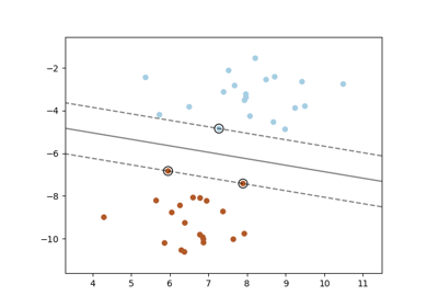
plot_training_data_with_decision_boundary("linear")
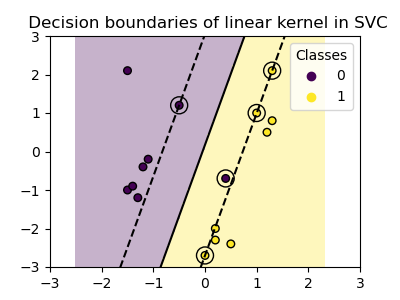
在具有线性核的SVC上进行训练会导致未转换的特征空间,其中超平面和边距是直线。由于线性核缺乏表达能力,训练出的类别不能完美地捕获训练数据。
多项式核#
多项式核改变了相似性的概念。核函数定义为
其中\({d}\)是多项式的次数(degree),\({\gamma}\)(gamma)控制每个单独训练样本对决策边界的影响,\({r}\)是偏置项(coef0),用于上下移动数据。在这里,我们使用核函数中多项式次数的默认值(degree=3)。当coef0=0(默认值)时,数据只进行转换,但不添加额外的维度。使用多项式核等效于创建PolynomialFeatures,然后在转换后的数据上拟合具有线性核的SVC,尽管对于大多数数据集来说,这种替代方法计算成本很高。
plot_training_data_with_decision_boundary("poly")
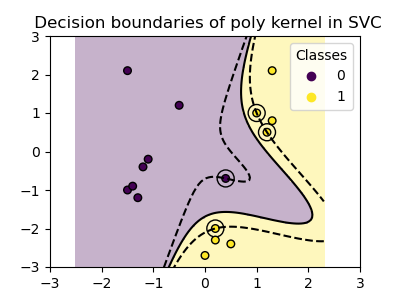
使用gamma=2的多项式核很好地适应了训练数据,导致超平面两侧的边距相应弯曲。
RBF核#
径向基函数(RBF)核,也称为高斯核,是scikit-learn中支持向量机的默认核函数。它在无限维度中测量两个数据点之间的相似性,然后通过多数投票进行分类。核函数定义为
其中\({\gamma}\)(gamma)控制每个单独训练样本对决策边界的影响。
两个点之间的欧几里得距离\(\|\mathbf{x}_1 - \mathbf{x}_2\|^2\)越大,核函数越接近零。这意味着相距很远的两个点更可能不相似。
plot_training_data_with_decision_boundary("rbf")
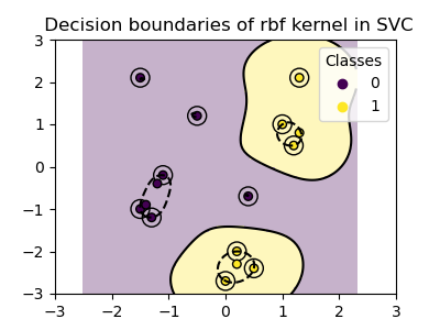
在图中我们可以看到决策边界如何倾向于收缩在彼此靠近的数据点周围。
S形核#
S形核函数定义为
其中核系数\({\gamma}\)(gamma)控制每个单独训练样本对决策边界的影响,\({r}\)是偏置项(coef0),用于上下移动数据。
在S形核中,使用双曲正切函数(\(\tanh\))计算两个数据点之间的相似性。核函数缩放并可能移动两个点(\(\mathbf{x}_1\)和\(\mathbf{x}_2\))的点积。
plot_training_data_with_decision_boundary("sigmoid")
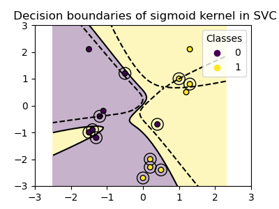
我们可以看到使用S形核获得的决策边界呈现弯曲且不规则的形状。决策边界试图通过拟合S形曲线来分离类别,导致一个复杂的边界,可能无法很好地推广到未见数据。从这个例子可以明显看出,S形核在处理具有S形形状的数据时具有非常特定的用例。在这个例子中,仔细微调可能会找到更具推广性的决策边界。由于其特殊性,S形核在实践中不如其他核函数常用。
结论#
在此示例中,我们可视化了使用提供的数据集训练的决策边界。这些图直观地展示了不同核函数如何利用训练数据来确定分类边界。
超平面和边距,尽管是间接计算的,可以想象为转换后特征空间中的平面。然而,在图中,它们是相对于原始特征空间表示的,导致多项式核、RBF核和S形核具有弯曲的决策边界。
请注意,这些图并未评估单个核函数的准确性或质量。它们旨在提供对不同核函数如何使用训练数据的视觉理解。
为了进行全面评估,建议使用GridSearchCV等技术对SVC参数进行微调,以捕获数据中的底层结构。
XOR数据集#
XOR模式是数据集非线性可分的经典示例。在这里,我们演示了不同的核函数如何在此类数据集上工作。
xx, yy = np.meshgrid(np.linspace(-3, 3, 500), np.linspace(-3, 3, 500))
np.random.seed(0)
X = np.random.randn(300, 2)
y = np.logical_xor(X[:, 0] > 0, X[:, 1] > 0)

_, ax = plt.subplots(2, 2, figsize=(8, 8))
args = dict(long_title=False, support_vectors=False)
plot_training_data_with_decision_boundary("linear", ax[0, 0], **args)
plot_training_data_with_decision_boundary("poly", ax[0, 1], **args)
plot_training_data_with_decision_boundary("rbf", ax[1, 0], **args)
plot_training_data_with_decision_boundary("sigmoid", ax[1, 1], **args)
plt.show()
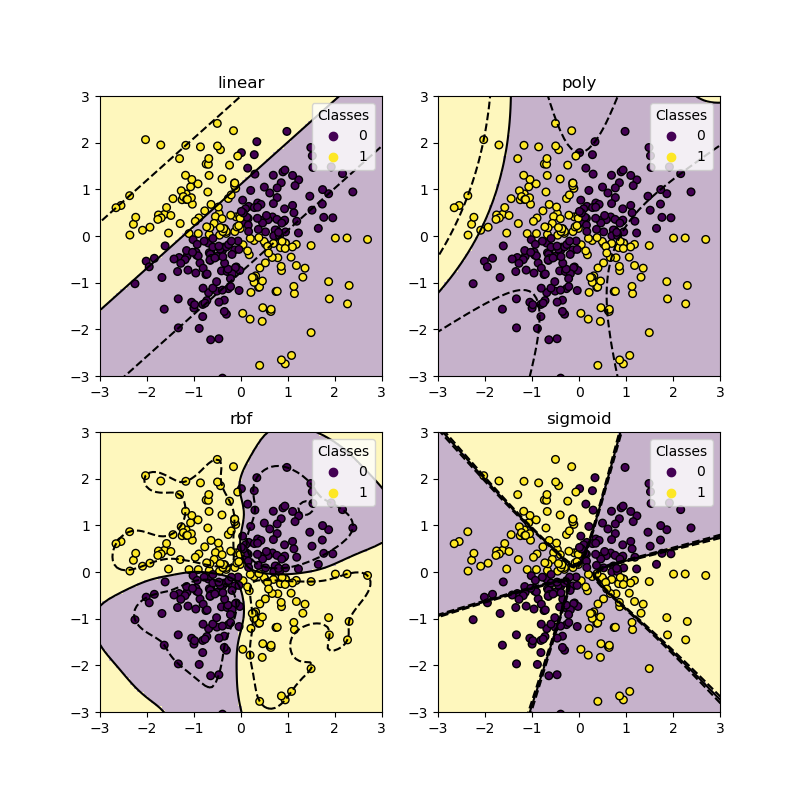
从上面的图中可以看出,只有rbf核能为上述数据集找到一个合理的决策边界。
脚本总运行时间: (0 minutes 1.151 seconds)
相关示例