注意
转到末尾 下载完整示例代码。或通过 JupyterLite 或 Binder 在浏览器中运行此示例
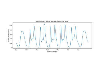
时间序列预测的滞后特征#
本示例演示了如何将 Polars 工程化的滞后特征用于 HistGradientBoostingRegressor 在共享单车需求数据集上的时间序列预测。
请参阅时间相关特征工程的示例,了解此数据集的一些数据探索和周期性特征工程演示。
# Authors: The scikit-learn developers
# SPDX-License-Identifier: BSD-3-Clause
分析共享单车需求数据集#
我们首先从 OpenML 仓库加载数据作为原始 parquet 文件,以说明如何处理任意 parquet 文件,而不是将此步骤隐藏在 sklearn.datasets.fetch_openml 等便捷工具中。
parquet 文件的 URL 可以在 openml.org 上 ID 为 44063 的共享单车需求数据集的 JSON 描述中找到(https://openml.org/search?type=data&status=active&id=44063)。
还提供了文件的 sha256 哈希值,以确保下载文件的完整性。
import numpy as np
import polars as pl

from sklearn.datasets import fetch_file

pl.Config.set_fmt_str_lengths(20)

bike_sharing_data_file = fetch_file(
    "https://data.openml.org/datasets/0004/44063/dataset_44063.pq",
    sha256="d120af76829af0d256338dc6dd4be5df4fd1f35bf3a283cab66a51c1c6abd06a",
)
bike_sharing_data_file
PosixPath('/home/circleci/scikit_learn_data/data.openml.org/datasets_0004_44063/dataset_44063.pq')
我们使用 Polars 加载 parquet 文件进行特征工程。Polars 会自动缓存多个表达式中重用的公共子表达式(如下面的 pl.col("count").shift(1))。更多信息请参阅 https://docs.polars.org.cn/user-guide/lazy/optimizations/。
df = pl.read_parquet(bike_sharing_data_file)
接下来,我们查看数据集的统计摘要,以便更好地理解我们正在处理的数据。
import polars.selectors as cs

summary = df.select(cs.numeric()).describe()
summary
让我们查看数据集中存在的季节 "fall"、"spring"、"summer" 和 "winter" 的计数,以确认它们是平衡的。
import matplotlib.pyplot as plt

df["season"].value_counts()
生成 Polars 工程化的滞后特征#
让我们考虑根据过去的需求预测下一小时需求的问题。由于需求是一个连续变量,直观上可以使用任何回归模型。然而,我们没有通常的 (X_train, y_train) 数据集。相反,我们只有按时间顺序组织的 y_train 需求数据。
lagged_df = df.select(
    "count",
    *[pl.col("count").shift(i).alias(f"lagged_count_{i}h") for i in [1, 2, 3]],
    lagged_count_1d=pl.col("count").shift(24),
    lagged_count_1d_1h=pl.col("count").shift(24 + 1),
    lagged_count_7d=pl.col("count").shift(7 * 24),
    lagged_count_7d_1h=pl.col("count").shift(7 * 24 + 1),
    lagged_mean_24h=pl.col("count").shift(1).rolling_mean(24),
    lagged_max_24h=pl.col("count").shift(1).rolling_max(24),
    lagged_min_24h=pl.col("count").shift(1).rolling_min(24),
    lagged_mean_7d=pl.col("count").shift(1).rolling_mean(7 * 24),
    lagged_max_7d=pl.col("count").shift(1).rolling_max(7 * 24),
    lagged_min_7d=pl.col("count").shift(1).rolling_min(7 * 24),
)
lagged_df.tail(10)
但是请注意,前几行有未定义的值,因为它们自己的过去是未知的。这取决于我们使用了多少滞后
lagged_df.head(10)
现在我们可以将滞后特征分离到矩阵 X 中,并将目标变量(要预测的计数)分离到相同第一维的数组 y 中。
lagged_df = lagged_df.drop_nulls()
X = lagged_df.drop("count")
y = lagged_df["count"]
print("X shape: {}\ny shape: {}".format(X.shape, y.shape))
X shape: (17210, 13)
y shape: (17210,)
下一小时共享单车需求回归的朴素评估#
让我们随机分割表格化数据集来训练一个梯度提升回归树 (GBRT) 模型,并使用平均绝对百分比误差 (MAPE) 进行评估。如果我们的模型旨在进行预测(即,从过去数据预测未来数据),我们不应使用晚于测试数据的训练数据。在时间序列机器学习中,“i.i.d”(独立同分布)假设不成立,因为数据点不是独立的,并且具有时间关系。
from sklearn.ensemble import HistGradientBoostingRegressor
from sklearn.model_selection import train_test_split

X_train, X_test, y_train, y_test = train_test_split(
    X, y, test_size=0.2, random_state=42
)

model = HistGradientBoostingRegressor().fit(X_train, y_train)
查看模型的性能。
from sklearn.metrics import mean_absolute_percentage_error

y_pred = model.predict(X_test)
mean_absolute_percentage_error(y_test, y_pred)
0.3889873516666431
下一小时预测的正确评估#
让我们使用适当的评估分割策略,该策略考虑数据集的时间结构,以评估模型预测未来数据点的能力(避免通过从训练集中的滞后特征读取值来作弊)。
from sklearn.model_selection import TimeSeriesSplit

ts_cv = TimeSeriesSplit(
    n_splits=3,  # to keep the notebook fast enough on common laptops
    gap=48,  # 2 days data gap between train and test
    max_train_size=10000,  # keep train sets of comparable sizes
    test_size=3000,  # for 2 or 3 digits of precision in scores
)
all_splits = list(ts_cv.split(X, y))
训练模型并根据 MAPE 评估其性能。
train_idx, test_idx = all_splits[0]
X_train, X_test = X[train_idx, :], X[test_idx, :]
y_train, y_test = y[train_idx], y[test_idx]

model = HistGradientBoostingRegressor().fit(X_train, y_train)
y_pred = model.predict(X_test)
mean_absolute_percentage_error(y_test, y_pred)
0.44300751539296973
通过混洗训练测试分割测量的泛化误差过于乐观。基于时间的分割的泛化可能更能代表回归模型的真实性能。让我们通过适当的交叉验证来评估误差评估的这种变异性。
from sklearn.model_selection import cross_val_score

cv_mape_scores = -cross_val_score(
    model, X, y, cv=ts_cv, scoring="neg_mean_absolute_percentage_error"
)
cv_mape_scores
array([0.44300752, 0.27772182, 0.3697178 ])
各分割间的变异性相当大!在实际应用中,建议使用更多的分割来更好地评估变异性。从现在开始,我们将报告平均交叉验证分数及其标准差。
print(f"CV MAPE: {cv_mape_scores.mean():.3f} ± {cv_mape_scores.std():.3f}")
CV MAPE: 0.363 ± 0.068
我们可以计算评估指标和损失函数的几种组合,这些组合在下面有所报告。
from collections import defaultdict

from sklearn.metrics import (
    make_scorer,
    mean_absolute_error,
    mean_pinball_loss,
    root_mean_squared_error,
)
from sklearn.model_selection import cross_validate


def consolidate_scores(cv_results, scores, metric):
    if metric == "MAPE":
        scores[metric].append(f"{value.mean():.2f} ± {value.std():.2f}")
    else:
        scores[metric].append(f"{value.mean():.1f} ± {value.std():.1f}")

    return scores


scoring = {
    "MAPE": make_scorer(mean_absolute_percentage_error),
    "RMSE": make_scorer(root_mean_squared_error),
    "MAE": make_scorer(mean_absolute_error),
    "pinball_loss_05": make_scorer(mean_pinball_loss, alpha=0.05),
    "pinball_loss_50": make_scorer(mean_pinball_loss, alpha=0.50),
    "pinball_loss_95": make_scorer(mean_pinball_loss, alpha=0.95),
}
loss_functions = ["squared_error", "poisson", "absolute_error"]
scores = defaultdict(list)
for loss_func in loss_functions:
    model = HistGradientBoostingRegressor(loss=loss_func)
    cv_results = cross_validate(
        model,
        X,
        y,
        cv=ts_cv,
        scoring=scoring,
        n_jobs=2,
    )
    time = cv_results["fit_time"]
    scores["loss"].append(loss_func)
    scores["fit_time"].append(f"{time.mean():.2f} ± {time.std():.2f} s")

    for key, value in cv_results.items():
        if key.startswith("test_"):
            metric = key.split("test_")[1]
            scores = consolidate_scores(cv_results, scores, metric)
通过分位数回归建模预测不确定性#
与其像最小二乘和泊松损失那样建模 \(Y|X\) 分布的期望值,不如尝试估计条件分布的分位数。
对于给定的数据点 \(x_i\),\(Y|X=x_i\) 预计是一个随机变量,因为我们预期租赁数量无法从特征中 100% 准确预测。它可能受到现有滞后特征未能充分捕捉的其他变量的影响。例如,下一小时是否会下雨无法从过去的小时共享单车租赁数据中完全预测。这就是我们所说的随机不确定性。
分位数回归使得在不对分布形状做强假设的情况下,能够更精细地描述该分布。
quantile_list = [0.05, 0.5, 0.95]

for quantile in quantile_list:
    model = HistGradientBoostingRegressor(loss="quantile", quantile=quantile)
    cv_results = cross_validate(
        model,
        X,
        y,
        cv=ts_cv,
        scoring=scoring,
        n_jobs=2,
    )
    time = cv_results["fit_time"]
    scores["fit_time"].append(f"{time.mean():.2f} ± {time.std():.2f} s")

    scores["loss"].append(f"quantile {int(quantile * 100)}")
    for key, value in cv_results.items():
        if key.startswith("test_"):
            metric = key.split("test_")[1]
            scores = consolidate_scores(cv_results, scores, metric)

scores_df = pl.DataFrame(scores)
scores_df
让我们看看使每个指标最小化的损失函数。
def min_arg(col):
    col_split = pl.col(col).str.split(" ")
    return pl.arg_sort_by(
        col_split.list.get(0).cast(pl.Float64),
        col_split.list.get(2).cast(pl.Float64),
    ).first()


scores_df.select(
    pl.col("loss").get(min_arg(col_name)).alias(col_name)
    for col_name in scores_df.columns
    if col_name != "loss"
)
即使由于数据集中的方差导致分数分布重叠,但正如预期,当 loss="squared_error" 时平均 RMSE 较低,而当 loss="absolute_error" 时平均 MAPE 较低。对于分位数 5 和 95 的平均弹珠损失也是如此。与 50 分位数损失对应的分数与通过最小化其他损失函数获得的分数重叠,MAE 也是如此。
对预测的定性观察#
现在我们可以可视化模型在第 5 百分位数、中位数和第 95 百分位数方面的性能。
all_splits = list(ts_cv.split(X, y))
train_idx, test_idx = all_splits[0]

X_train, X_test = X[train_idx, :], X[test_idx, :]
y_train, y_test = y[train_idx], y[test_idx]

max_iter = 50
gbrt_mean_poisson = HistGradientBoostingRegressor(loss="poisson", max_iter=max_iter)
gbrt_mean_poisson.fit(X_train, y_train)
mean_predictions = gbrt_mean_poisson.predict(X_test)

gbrt_median = HistGradientBoostingRegressor(
    loss="quantile", quantile=0.5, max_iter=max_iter
)
gbrt_median.fit(X_train, y_train)
median_predictions = gbrt_median.predict(X_test)

gbrt_percentile_5 = HistGradientBoostingRegressor(
    loss="quantile", quantile=0.05, max_iter=max_iter
)
gbrt_percentile_5.fit(X_train, y_train)
percentile_5_predictions = gbrt_percentile_5.predict(X_test)

gbrt_percentile_95 = HistGradientBoostingRegressor(
    loss="quantile", quantile=0.95, max_iter=max_iter
)
gbrt_percentile_95.fit(X_train, y_train)
percentile_95_predictions = gbrt_percentile_95.predict(X_test)
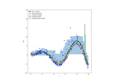
现在我们可以查看回归模型做出的预测。
last_hours = slice(-96, None)
fig, ax = plt.subplots(figsize=(15, 7))
plt.title("Predictions by regression models")
ax.plot(
    y_test[last_hours],
    "x-",
    alpha=0.2,
    label="Actual demand",
    color="black",
)
ax.plot(
    median_predictions[last_hours],
    "^-",
    label="GBRT median",
)
ax.plot(
    mean_predictions[last_hours],
    "x-",
    label="GBRT mean (Poisson)",
)
ax.fill_between(
    np.arange(96),
    percentile_5_predictions[last_hours],
    percentile_95_predictions[last_hours],
    alpha=0.3,
    label="GBRT 90% interval",
)
_ = ax.legend()
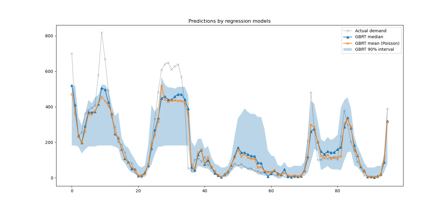
这里有趣的是,5% 和 95% 百分位数估计器之间的蓝色区域的宽度随一天中的时间而变化。
在夜间,蓝色区域窄得多:这对模型相当确信共享单车租赁数量会很小。而且,实际需求保持在该蓝色区域内,这似乎是正确的。
在白天,蓝色区域宽得多:不确定性增加,这可能是由于天气变化可能产生非常大的影响,尤其是在周末。
我们还可以看到,在工作日期间,通勤模式在 5% 和 95% 的估计中仍然可见。
最后,预计有 10% 的时间,实际需求不在 5% 和 95% 百分位数估计之间。在此测试范围内,实际需求似乎更高,尤其是在高峰时段。这可能表明我们的 95% 百分位数估计器低估了需求峰值。这可以通过计算经验覆盖率来定量证实,如置信区间校准中所做的那样。
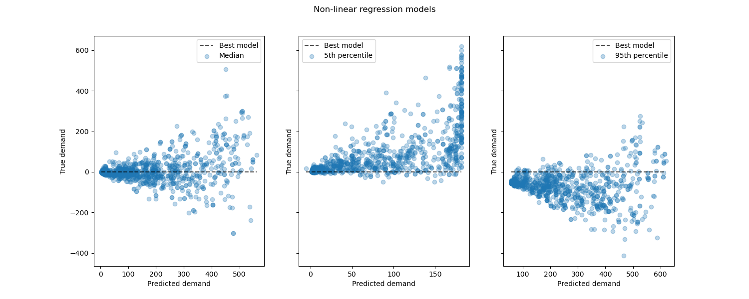
查看非线性回归模型与最佳模型的性能
from sklearn.metrics import PredictionErrorDisplay

fig, axes = plt.subplots(ncols=3, figsize=(15, 6), sharey=True)
fig.suptitle("Non-linear regression models")
predictions = [
    median_predictions,
    percentile_5_predictions,
    percentile_95_predictions,
]
labels = [
    "Median",
    "5th percentile",
    "95th percentile",
]
for ax, pred, label in zip(axes, predictions, labels):
    PredictionErrorDisplay.from_predictions(
        y_true=y_test,
        y_pred=pred,
        kind="residual_vs_predicted",
        scatter_kwargs={"alpha": 0.3},
        ax=ax,
    )
    ax.set(xlabel="Predicted demand", ylabel="True demand")
    ax.legend(["Best model", label])

plt.show()
结论#
通过本示例,我们探索了使用滞后特征进行时间序列预测。我们将朴素回归(使用标准化的 train_test_split)与使用 TimeSeriesSplit 的正确时间序列评估策略进行了比较。我们观察到,使用 train_test_split(其中 shuffle 的默认值为 True)训练的模型产生了过于乐观的平均绝对百分比误差 (MAPE)。基于时间的分割产生的结果更能代表我们时间序列回归模型的真实性能。我们还通过分位数回归分析了模型的预测不确定性。使用 loss="quantile" 进行的基于第 5 和第 95 百分位数的预测,为我们时间序列回归模型所做预测的不确定性提供了定量估计。不确定性估计也可以使用 MAPIE 来执行,它提供了一个基于保形预测方法的最新工作的实现,同时估计随机不确定性(aleatoric uncertainty)和认知不确定性(epistemic uncertainty)。此外,sktime 提供的功能可用于通过递归时间序列预测扩展 scikit-learn 估计器,从而实现未来值的动态预测。
脚本总运行时间: (0 分 9.613 秒)
相关示例