注意

跳到最后下载完整的示例代码，或通过 JupyterLite 或 Binder 在浏览器中运行此示例

类似然比衡量分类性能#

本示例演示了 class_likelihood_ratios 函数，该函数计算正似然比和负似然比（LR+，LR-）以评估二分类器的预测能力。我们将看到，这些指标独立于测试集中的类别比例，这使得它们在研究的可用数据与目标应用具有不同类别比例时非常有用。

一个典型的应用是医学中的病例对照研究，其中类别几乎平衡，而一般人群则存在较大的类别不平衡。在这种应用中，个体患目标疾病的先验概率可以选择为患病率，即在特定人群中发现受某种疾病影响的比例。后验概率则表示在测试结果为阳性时，该疾病确实存在的概率。

在本示例中，我们首先讨论由类似然比给出的先验几率和后验几率之间的联系。然后，我们在一些受控场景中评估它们的行为。在最后一部分中，我们将它们绘制为正类别患病率的函数。

# Authors: The scikit-learn developers
# SPDX-License-Identifier: BSD-3-Clause

先验与后验分析#

假设我们有一个人群，他们具有生理测量值 X，有望作为疾病的间接生物标志物，以及实际疾病指标 y（真实标签）。人群中的大多数人没有携带疾病，但少数人（本例中约为 10%）携带。

from sklearn.datasets import make_classification

X, y = make_classification(n_samples=10_000, weights=[0.9, 0.1], random_state=0)
print(f"Percentage of people carrying the disease: {100 * y.mean():.2f}%")

Percentage of people carrying the disease: 10.37%

构建了一个机器学习模型来诊断具有给定生理测量值的人是否可能携带感兴趣的疾病。为了评估模型，我们需要在保留的测试集上评估其性能。

from sklearn.model_selection import train_test_split

X_train, X_test, y_train, y_test = train_test_split(X, y, random_state=0)

然后我们可以拟合我们的诊断模型并计算正似然比，以评估此分类器作为疾病诊断工具的实用性。

from sklearn.linear_model import LogisticRegression
from sklearn.metrics import class_likelihood_ratios

estimator = LogisticRegression().fit(X_train, y_train)
y_pred = estimator.predict(X_test)
pos_LR, neg_LR = class_likelihood_ratios(y_test, y_pred, replace_undefined_by=1.0)
print(f"LR+: {pos_LR:.3f}")

LR+: 12.617

由于正类别似然比远大于 1.0，这意味着基于机器学习的诊断工具是有用的：在测试结果为阳性时，疾病确实存在的后验几率是先验几率的 12 倍以上。

似然比的交叉验证#

我们评估在某些特定情况下，类别似然比测量值的变异性。

import pandas as pd


def scoring(estimator, X, y):
    y_pred = estimator.predict(X)
    pos_lr, neg_lr = class_likelihood_ratios(y, y_pred, replace_undefined_by=1.0)
    return {"positive_likelihood_ratio": pos_lr, "negative_likelihood_ratio": neg_lr}


def extract_score(cv_results):
    lr = pd.DataFrame(
        {
            "positive": cv_results["test_positive_likelihood_ratio"],
            "negative": cv_results["test_negative_likelihood_ratio"],
        }
    )
    return lr.aggregate(["mean", "std"])

我们首先使用上一节中使用的默认超参数验证 LogisticRegression 模型。

from sklearn.model_selection import cross_validate

estimator = LogisticRegression()
extract_score(cross_validate(estimator, X, y, scoring=scoring, cv=10))

	正类	负类
均值	16.661086	0.724702
标准差	4.383973	0.054045

我们确认该模型是有用的：后验几率是先验几率的 12 到 20 倍。

相反，让我们考虑一个虚拟模型，它将输出与训练集中平均疾病患病率相似几率的随机预测。

from sklearn.dummy import DummyClassifier

estimator = DummyClassifier(strategy="stratified", random_state=1234)
extract_score(cross_validate(estimator, X, y, scoring=scoring, cv=10))

	正类	负类
均值	1.108843	0.986989
标准差	0.268147	0.034278

这里两个类别似然比都与 1.0 兼容，这使得该分类器作为改善疾病检测的诊断工具毫无用处。

虚拟模型的另一个选择是始终预测最常见的类别，在这种情况下是“无病”。

estimator = DummyClassifier(strategy="most_frequent")
extract_score(cross_validate(estimator, X, y, scoring=scoring, cv=10))

/home/circleci/project/sklearn/utils/_param_validation.py:218: UndefinedMetricWarning:

No samples were predicted for the positive class and `positive_likelihood_ratio` is set to `np.nan`. Use the `replace_undefined_by` param to

/home/circleci/project/sklearn/utils/_param_validation.py:218: UndefinedMetricWarning:

No samples were predicted for the positive class and `positive_likelihood_ratio` is set to `np.nan`. Use the `replace_undefined_by` param to

/home/circleci/project/sklearn/utils/_param_validation.py:218: UndefinedMetricWarning:

No samples were predicted for the positive class and `positive_likelihood_ratio` is set to `np.nan`. Use the `replace_undefined_by` param to

/home/circleci/project/sklearn/utils/_param_validation.py:218: UndefinedMetricWarning:

No samples were predicted for the positive class and `positive_likelihood_ratio` is set to `np.nan`. Use the `replace_undefined_by` param to

/home/circleci/project/sklearn/utils/_param_validation.py:218: UndefinedMetricWarning:

No samples were predicted for the positive class and `positive_likelihood_ratio` is set to `np.nan`. Use the `replace_undefined_by` param to

/home/circleci/project/sklearn/utils/_param_validation.py:218: UndefinedMetricWarning:

No samples were predicted for the positive class and `positive_likelihood_ratio` is set to `np.nan`. Use the `replace_undefined_by` param to

/home/circleci/project/sklearn/utils/_param_validation.py:218: UndefinedMetricWarning:

No samples were predicted for the positive class and `positive_likelihood_ratio` is set to `np.nan`. Use the `replace_undefined_by` param to

/home/circleci/project/sklearn/utils/_param_validation.py:218: UndefinedMetricWarning:

No samples were predicted for the positive class and `positive_likelihood_ratio` is set to `np.nan`. Use the `replace_undefined_by` param to

/home/circleci/project/sklearn/utils/_param_validation.py:218: UndefinedMetricWarning:

No samples were predicted for the positive class and `positive_likelihood_ratio` is set to `np.nan`. Use the `replace_undefined_by` param to

/home/circleci/project/sklearn/utils/_param_validation.py:218: UndefinedMetricWarning:

No samples were predicted for the positive class and `positive_likelihood_ratio` is set to `np.nan`. Use the `replace_undefined_by` param to

	正类	负类
均值	1.0	1.0
标准差	0.0	0.0

没有正向预测意味着没有真阳性也没有假阳性，导致 LR+ 未定义，这绝不应被解释为无限大的 LR+（分类器完美识别阳性病例）。在这种情况下，class_likelihood_ratios 函数默认返回 nan 并发出警告。实际上，LR- 的值有助于我们排除此模型。

当对样本量较少且高度不平衡的数据进行交叉验证时，可能会出现类似的情况：某些折叠中没有患病样本，因此在用于测试时它们不会输出真阳性或假阴性。从数学上讲，这会导致 LR+ 无限大，这也不应被解释为模型完美识别阳性病例。此类事件会导致估计似然比的方差更高，但仍可解释为患病后验几率的增加。

estimator = LogisticRegression()
X, y = make_classification(n_samples=300, weights=[0.9, 0.1], random_state=0)
extract_score(cross_validate(estimator, X, y, scoring=scoring, cv=10))

/home/circleci/project/sklearn/utils/_param_validation.py:218: UndefinedMetricWarning:

`positive_likelihood_ratio` is ill-defined and set to `np.nan`. Use the `replace_undefined_by` param to

/home/circleci/project/sklearn/utils/_param_validation.py:218: UndefinedMetricWarning:

`positive_likelihood_ratio` is ill-defined and set to `np.nan`. Use the `replace_undefined_by` param to

/home/circleci/project/sklearn/utils/_param_validation.py:218: UndefinedMetricWarning:

`positive_likelihood_ratio` is ill-defined and set to `np.nan`. Use the `replace_undefined_by` param to

/home/circleci/project/sklearn/utils/_param_validation.py:218: UndefinedMetricWarning:

`positive_likelihood_ratio` is ill-defined and set to `np.nan`. Use the `replace_undefined_by` param to

/home/circleci/project/sklearn/utils/_param_validation.py:218: UndefinedMetricWarning:

`positive_likelihood_ratio` is ill-defined and set to `np.nan`. Use the `replace_undefined_by` param to

	正类	负类
均值	9.400000	0.373333
标准差	10.532489	0.235430

关于患病率的不变性#

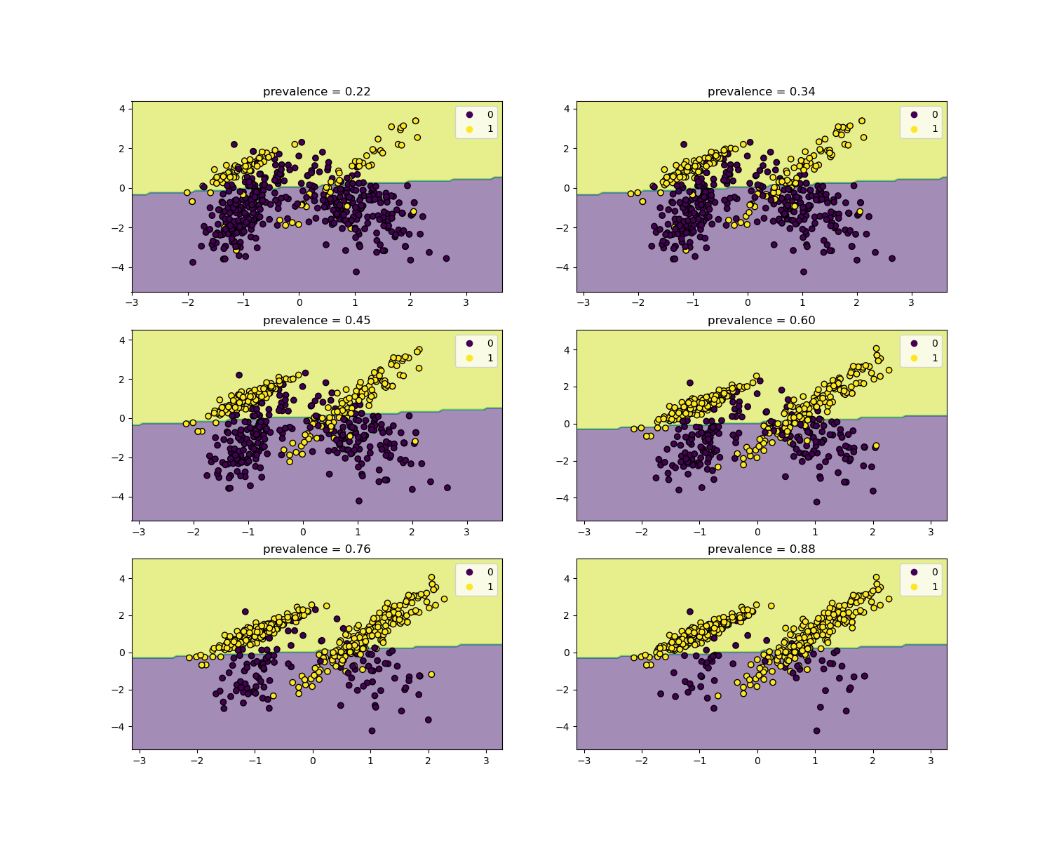
似然比独立于疾病患病率，并且可以在不同人群之间进行外推，无论是否存在类别不平衡，只要对所有人群应用相同的模型。请注意，在下面的图中，决策边界是常数（有关非平衡类别边界决策的研究，请参阅 SVM：非平衡类的分离超平面）。

在这里，我们在一个患病率为 50% 的病例对照研究中训练一个 LogisticRegression 基础模型。然后，在患病率不同的人群上进行评估。我们使用 make_classification 函数来确保数据生成过程始终与下图所示相同。标签 1 对应正类别“疾病”，而标签 0 代表“无病”。

from collections import defaultdict

import matplotlib.pyplot as plt
import numpy as np

from sklearn.inspection import DecisionBoundaryDisplay

populations = defaultdict(list)
common_params = {
    "n_samples": 10_000,
    "n_features": 2,
    "n_informative": 2,
    "n_redundant": 0,
    "random_state": 0,
}
weights = np.linspace(0.1, 0.8, 6)
weights = weights[::-1]

# fit and evaluate base model on balanced classes
X, y = make_classification(**common_params, weights=[0.5, 0.5])
estimator = LogisticRegression().fit(X, y)
lr_base = extract_score(cross_validate(estimator, X, y, scoring=scoring, cv=10))
pos_lr_base, pos_lr_base_std = lr_base["positive"].values
neg_lr_base, neg_lr_base_std = lr_base["negative"].values

现在我们将展示每个患病率水平的决策边界。请注意，我们只绘制了原始数据的一个子集，以便更好地评估线性模型的决策边界。

fig, axs = plt.subplots(nrows=3, ncols=2, figsize=(15, 12))

for ax, (n, weight) in zip(axs.ravel(), enumerate(weights)):
    X, y = make_classification(
        **common_params,
        weights=[weight, 1 - weight],
    )
    prevalence = y.mean()
    populations["prevalence"].append(prevalence)
    populations["X"].append(X)
    populations["y"].append(y)

    # down-sample for plotting
    rng = np.random.RandomState(1)
    plot_indices = rng.choice(np.arange(X.shape[0]), size=500, replace=True)
    X_plot, y_plot = X[plot_indices], y[plot_indices]

    # plot fixed decision boundary of base model with varying prevalence
    disp = DecisionBoundaryDisplay.from_estimator(
        estimator,
        X_plot,
        response_method="predict",
        alpha=0.5,
        ax=ax,
    )
    scatter = disp.ax_.scatter(X_plot[:, 0], X_plot[:, 1], c=y_plot, edgecolor="k")
    disp.ax_.set_title(f"prevalence = {y_plot.mean():.2f}")
    disp.ax_.legend(*scatter.legend_elements())

prevalence = 0.22, prevalence = 0.34, prevalence = 0.45, prevalence = 0.60, prevalence = 0.76, prevalence = 0.88

我们定义一个用于自举的函数。

def scoring_on_bootstrap(estimator, X, y, rng, n_bootstrap=100):
    results_for_prevalence = defaultdict(list)
    for _ in range(n_bootstrap):
        bootstrap_indices = rng.choice(
            np.arange(X.shape[0]), size=X.shape[0], replace=True
        )
        for key, value in scoring(
            estimator, X[bootstrap_indices], y[bootstrap_indices]
        ).items():
            results_for_prevalence[key].append(value)
    return pd.DataFrame(results_for_prevalence)

我们使用自举为每个患病率对基础模型进行评分。

results = defaultdict(list)
n_bootstrap = 100
rng = np.random.default_rng(seed=0)

for prevalence, X, y in zip(
    populations["prevalence"], populations["X"], populations["y"]
):
    results_for_prevalence = scoring_on_bootstrap(
        estimator, X, y, rng, n_bootstrap=n_bootstrap
    )
    results["prevalence"].append(prevalence)
    results["metrics"].append(
        results_for_prevalence.aggregate(["mean", "std"]).unstack()
    )

results = pd.DataFrame(results["metrics"], index=results["prevalence"])
results.index.name = "prevalence"
results

	正似然比		负似然比
	均值	标准差	均值	标准差
患病率
0.2039	4.507943	0.113516	0.207667	0.009778
0.3419	4.443238	0.125140	0.198766	0.008915
0.4809	4.421087	0.123828	0.192913	0.006360
0.6196	4.409717	0.164009	0.193949	0.005861
0.7578	4.334795	0.175298	0.189267	0.005840
0.8963	4.197666	0.238955	0.185654	0.005027

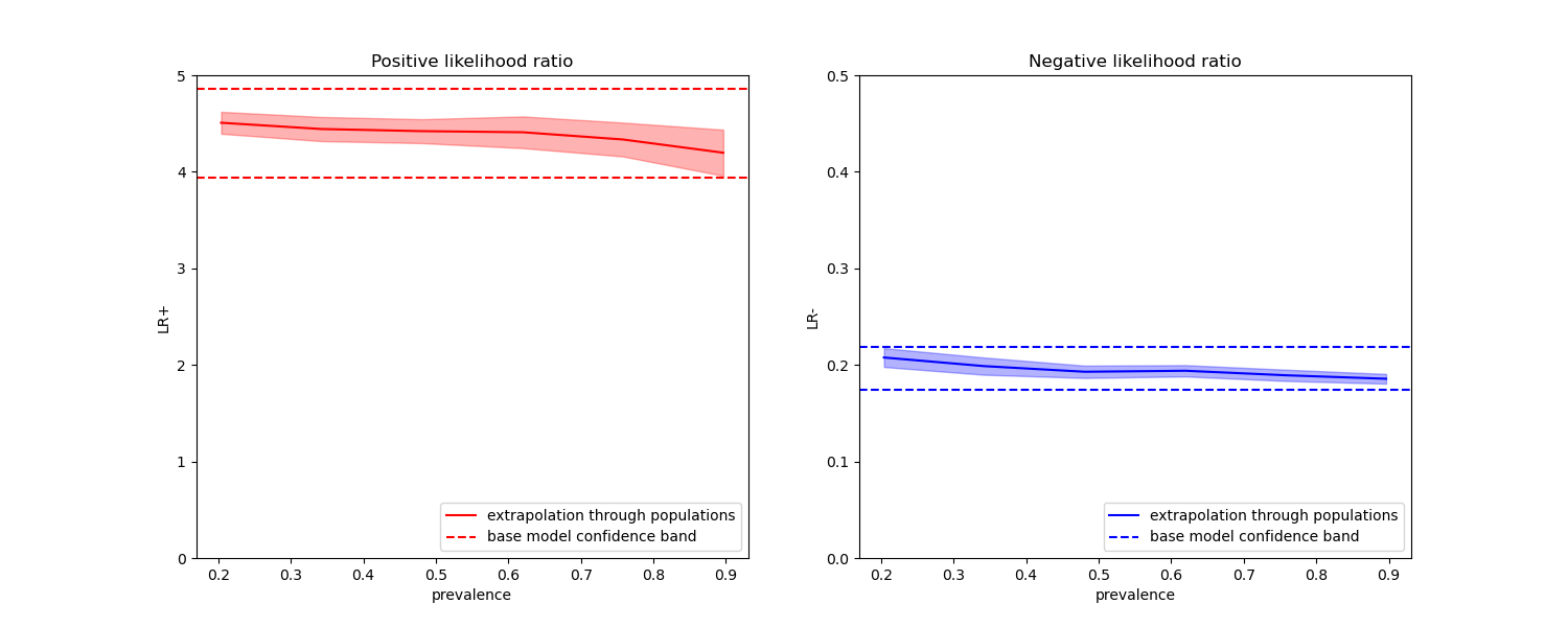
在下面的图中，我们观察到使用不同患病率重新计算的类别似然比在与平衡类别计算出的结果的一个标准差范围内确实是常数。

fig, (ax1, ax2) = plt.subplots(nrows=1, ncols=2, figsize=(15, 6))
results["positive_likelihood_ratio"]["mean"].plot(
    ax=ax1, color="r", label="extrapolation through populations"
)
ax1.axhline(y=pos_lr_base + pos_lr_base_std, color="r", linestyle="--")
ax1.axhline(
    y=pos_lr_base - pos_lr_base_std,
    color="r",
    linestyle="--",
    label="base model confidence band",
)
ax1.fill_between(
    results.index,
    results["positive_likelihood_ratio"]["mean"]
    - results["positive_likelihood_ratio"]["std"],
    results["positive_likelihood_ratio"]["mean"]
    + results["positive_likelihood_ratio"]["std"],
    color="r",
    alpha=0.3,
)
ax1.set(
    title="Positive likelihood ratio",
    ylabel="LR+",
    ylim=[0, 5],
)
ax1.legend(loc="lower right")

ax2 = results["negative_likelihood_ratio"]["mean"].plot(
    ax=ax2, color="b", label="extrapolation through populations"
)
ax2.axhline(y=neg_lr_base + neg_lr_base_std, color="b", linestyle="--")
ax2.axhline(
    y=neg_lr_base - neg_lr_base_std,
    color="b",
    linestyle="--",
    label="base model confidence band",
)
ax2.fill_between(
    results.index,
    results["negative_likelihood_ratio"]["mean"]
    - results["negative_likelihood_ratio"]["std"],
    results["negative_likelihood_ratio"]["mean"]
    + results["negative_likelihood_ratio"]["std"],
    color="b",
    alpha=0.3,
)
ax2.set(
    title="Negative likelihood ratio",
    ylabel="LR-",
    ylim=[0, 0.5],
)
ax2.legend(loc="lower right")

plt.show()

Positive likelihood ratio, Negative likelihood ratio

脚本总运行时间： (0 分钟 1.741 秒)

类似然比衡量分类性能#

先验与后验分析#

似然比的交叉验证#

关于患病率的不变性#

本页